These are the lecture notes for FAU’s YouTube Lecture “Medical Engineering“. This is a full transcript of the lecture video & matching slides. We hope, you enjoy this as much as the videos. Of course, this transcript was created with deep learning techniques largely automatically and only minor manual modifications were performed. Try it yourself! If you spot mistakes, please let us know!
Welcome back to Medical Engineering. So today we want to talk a little bit about a new kind of modality. This is called X-ray phase-contrast imaging. So in the following video, we want to talk a bit about whether X-rays are particles or, waves. We’ll see that there are also wave characteristics that we can use to determine phase contrast and related contrasts. So looking forward to exploring a little bit more of X-ray physics with you guys.
So we start with a little motivation. Let’s have a look at what we can find with the phase-contrast images.
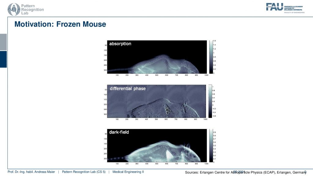
So this is the absorption image. So you’ve already seen that for quite some time and we know that this is essentially just the absorption effect just a regular X-ray image. You see that we see bones here very well and this is a mouse that you can see here in this image. But there’s more to that. There is the so-called differential phase and this is measuring the phase shift and here we get a very different contrast and to be honest we get a derivative with respect to x-direction that is reconstructed. You see that we see the very fine structures here in the lung. Yet we have a third modality here and the third modality is the so-called dark-field image. This is a very different contrast than what we had in mind so far because this is reacting to structures. So you can see here that it reacts to the lung and it reacts here to the skin of the mouse but it’s actually not the skin. It’s the fur. So it’s the tiny hair that is growing on the mouse and this causes a large signal that we can see here in this image. So to be honest the dark field image is measuring micro angle scatter. So we can see scatter that is actually caused by microstructures that are in the range of micrometers. So here are the hairs and also the very small and fine structures the small bubbles in the lung that cause this high contrast in this image. So you see this is a completely new contrast and we think that it may become highly relevant with respect to medical diagnosis.
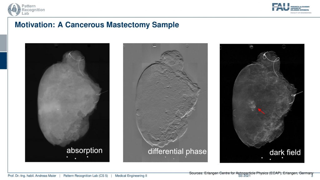
So we have a kind of overview image here where we show again the three different contrasts for a different kind of object. Here this is a mastectomy. So we removed the breast in the case of cancer and then we looked at the breast with the different modalities. Here you can see first of all somethings is appearing in the face contrast image. But more importantly, you see these small shadows that don’t show up in any of the other two images. We think that this is related to microcalcifications which are indicative of early cancer development. So here phase contrast and darkfield images may be game-changers for the diagnosis of breast cancer.
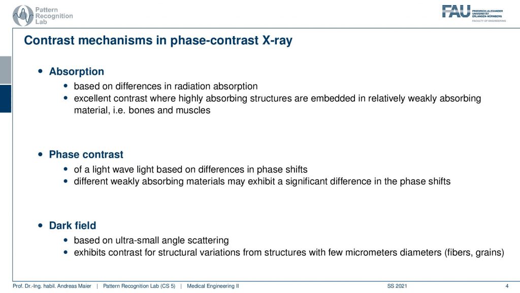
So what do we see in these images? Let’s summarize this. In the absorption image, we see differences in radiation absorption. In the phase contrast image, we see the differences in phase shifts. In the dark field, we see the ultra small-angle scattering that is caused by microscopic structures that are way smaller than the actual detector pixel or the reconstruction voxel grid. So we can measure effects that are an order of magnitude smaller than the actual reconstruction takes place on. So this is pretty interesting and we’ll see some very interesting results towards the end of this video.
Now let’s discuss a little bit why we can use the wave characteristics in order to get contrast.
The key element that we want to look at here is interference.
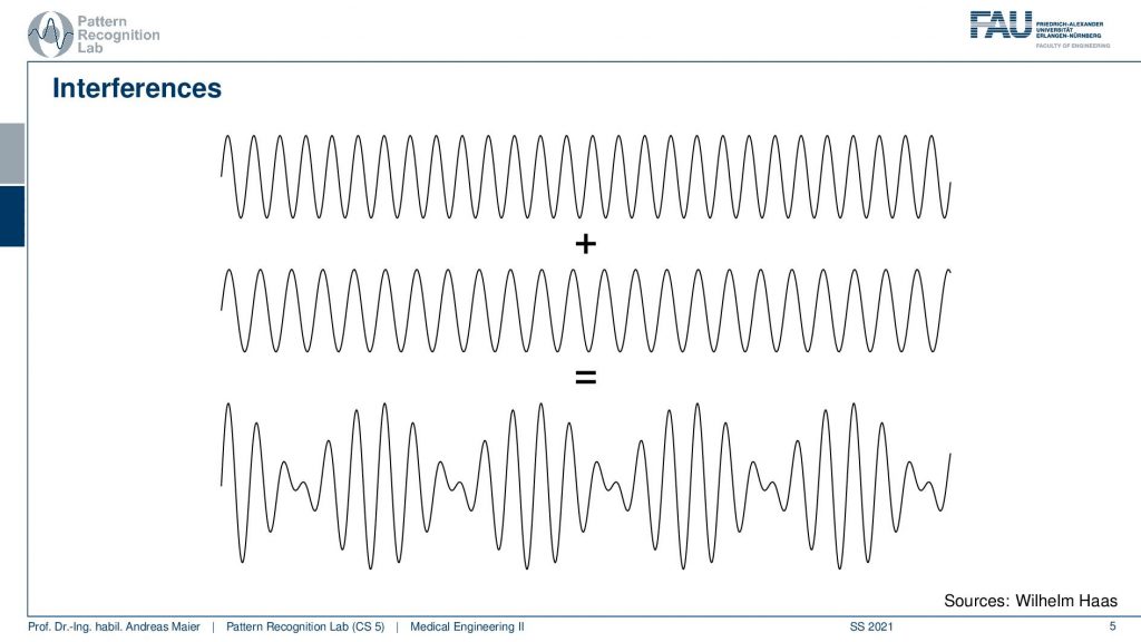
We can get interference between two waves if we add them and here is an example with two different wavelengths. You can see that at some places it actually causes constructive interference and at other places, they cancel out and there is a loss of signal. Unfortunately, this is not stationary and it moves along with the waves. So we don’t have a stable interference here. If you want to achieve stable interference, you need waves of the same wavelength.
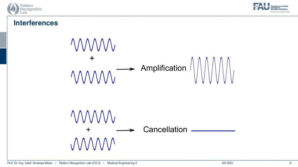
So they have the same wavelength and they will amplify exactly in the cases where they are in synchrony. So here you get stronger signals because the wavelength is exactly in phase. In order to get a cancellation, you have to have the signal in a position where the wavelength is shifted by half a wavelength and if that happens then you will get a cancellation. So you see that the positive and the negative parts here always oppose each other and this causes a cancellation here when the two waves are superimposed.
So we learned that for stationary interference we need these two waves and they have to be at the same frequency. Then we have a constant phase shift. If we have a constant phase shift we get exactly this cancellation and also constructive interference patterns that we then can observe as white and black peaks.
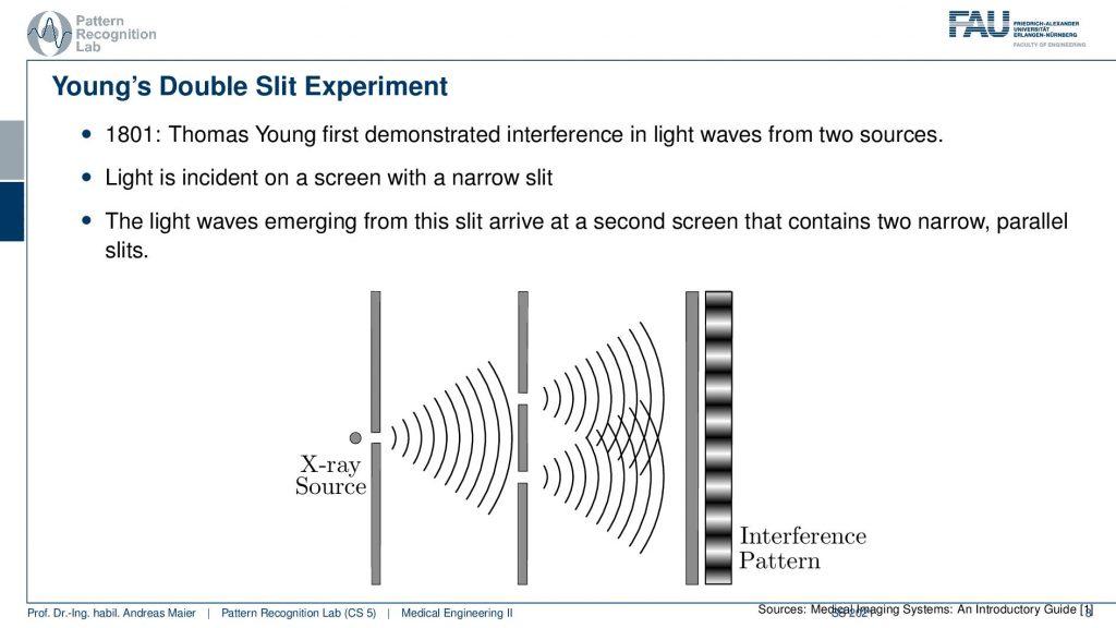
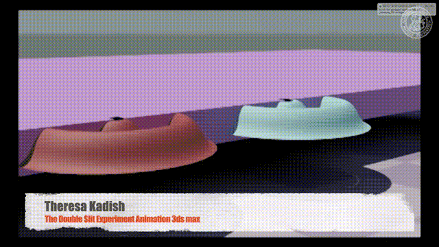
So if we want to construct this we have to use a geometric setup that is called Young’s double-slit experiment. In 1801 Thomas Young discovered this kind of experiment with two slits and visible light. He demonstrated that you can construct interference patterns and these interference patterns form white and black fringes here if you use two slits and they’re approximately in the same distance. In order to do that you need one light source that is emitting essentially a wavefront here and by the double-slit essentially the wavefront copies and this causes then the interference pattern. So Young showed this with visible light. But we can construct similar stuff also with X-rays and we’ll see that it’s a bit more complicated to construct it. But technically we can also use this effect to get a signal.
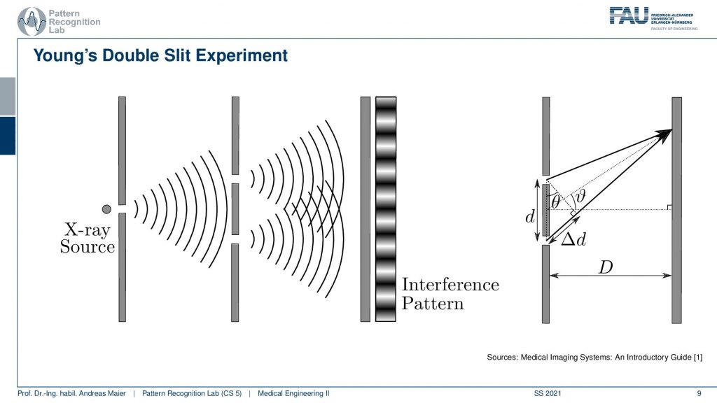
Now what is actually relevant is the distance that is the difference in the actual phase. So we are actually interested in a ∆ and this ∆ then constructs the positive and negative interference patterns of the black and white fringes. In order to determine this, you have to know the distance between the two slits and this angle here because this angle here is driving the ∆d. From the angle here and the distance, I can compute the ∆d and if I have a ∆d that is exactly one wavelength or zero then I will have the constructive interference and if I have half a wavelength the two waves will cancel out. So that’s the key observation that we need to keep in mind.
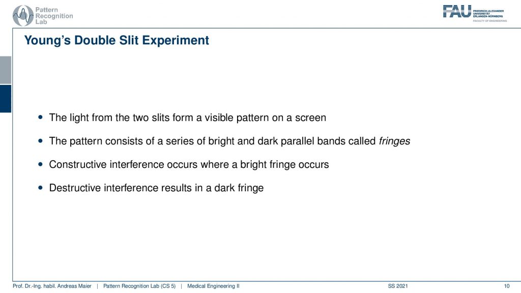
So let’s summarize this. The light from the two slits forms a visible pattern on the screen. The pattern consists of a series of bright and dark parallel bands called fringes. The constructive interference patterns occur when a bright fringe is there. The destructive interference pattern is a dark fringe. Now how is this constructed?
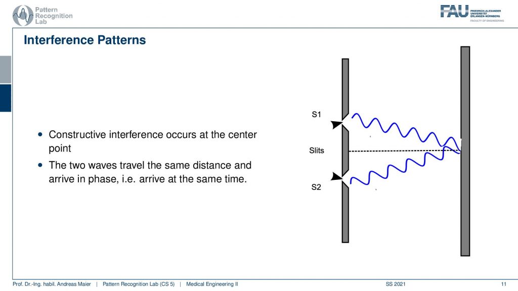
we can visualize this here. So if we have the same distance in terms of the wave propagating from here to here and from here to here then they will be in sync. So if I have a wave running around here then you will see that I get the same kind of observation here and the two waves will actually start to interfere in a constructive manner.
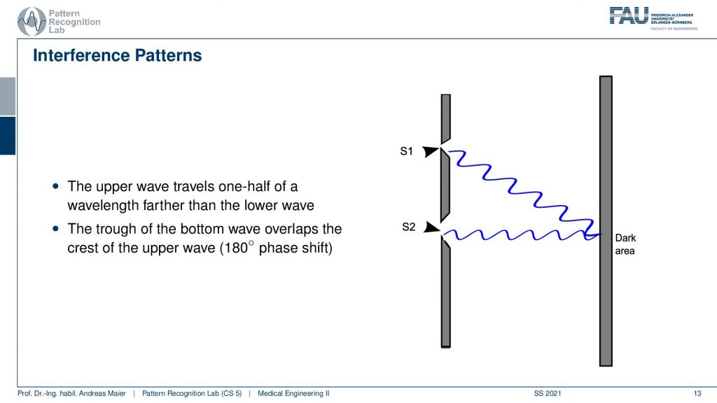
If I have half a wavelength in between then I can also create an interference pattern. Here you actually see that in this particular kind of setup we have a different length here and a different length here and this then means that also our waves have to travel over different distances. Here you see exactly that this kind of interference appears and now that I’ve drawn it, it’s actually not a bright area. So this is a dark area that appears here because of the way I’ve drawn it. Obviously, this would be half a wavelength of shift and there can be also the other case where you have then exactly one additional wavelength of shift.
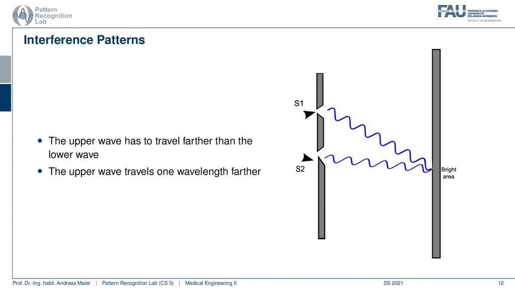
If I choose my wavelength again in the same way then you will see that I get exactly one more wave up there but they still intersect at the point where they have essentially the same phase shift. Then we have a bright fringe appearing here. So this is how the constructive and the destructive patterns emerge.
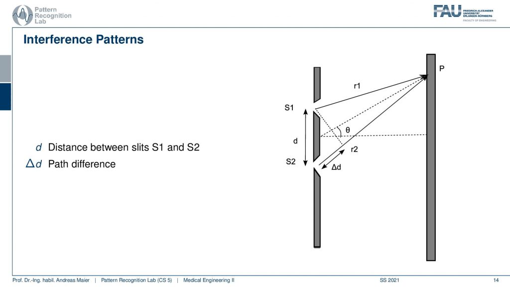
We can now summarize this. If we formalize over ∆d, ∆ and our angle and the two distances r1 and r2 then we can set this up into an equation.
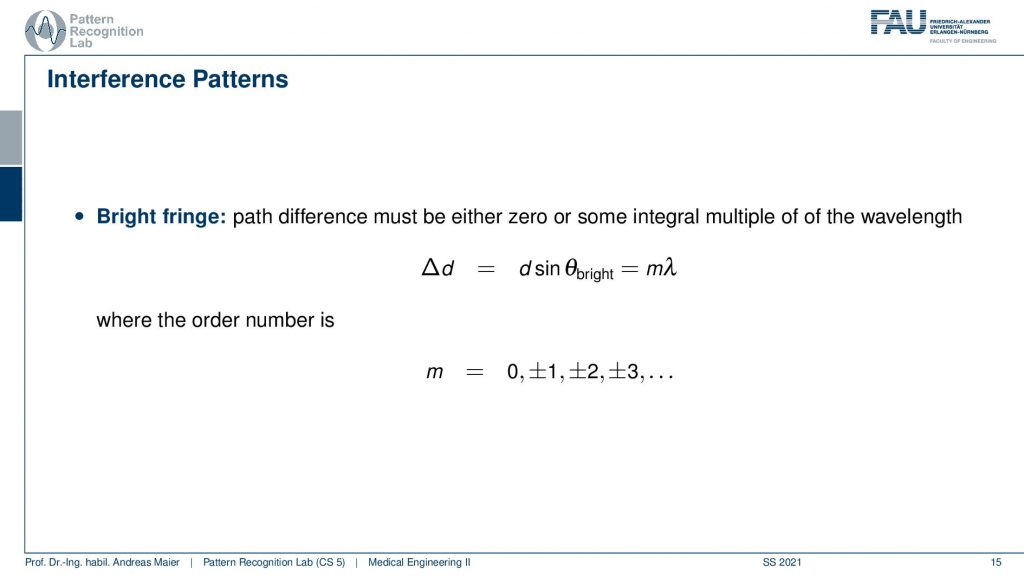
So ∆d is given as d times sinθ and if the case is d times sinθ is m times λ. Here m is an integer value. If this is exactly an integer you will have the bright fringe.
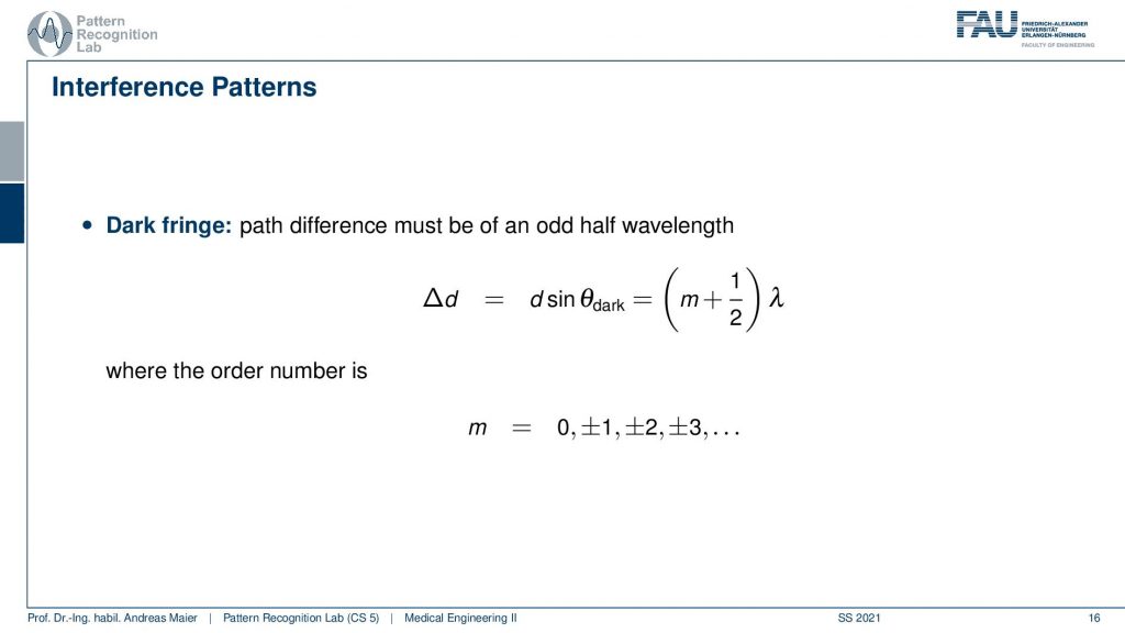
If the pattern is shifted by half a wavelength and again m is an integer you get the dark fringe. So this is the main result that explains to us how we are actually constructing these kinds of positive and negative interference patterns and how the bright and dark fringes emerge.
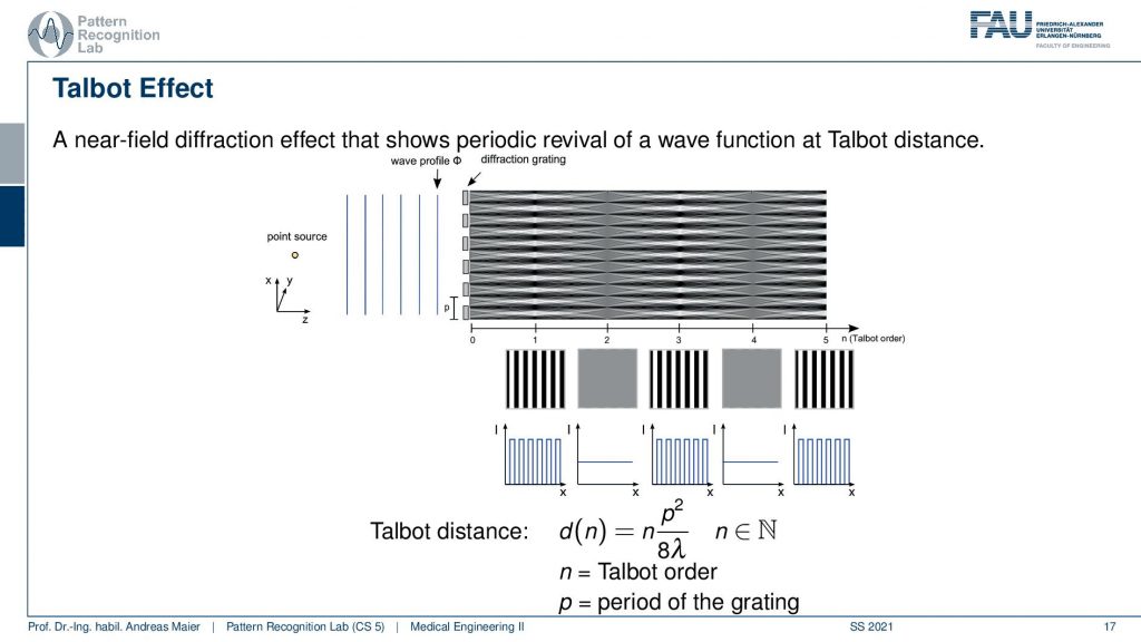
There’s a little more to that because these interference patterns don’t appear at arbitrary distances. They actually appear at certain distances which are called the Talbot effect. This is Talbot distance and the Talbot distance tells us essentially that if I’m exactly in a talbot distance of 1, I observe the interference pattern. But at the table distance times 2. There’s exactly nothing just gray and no interference pattern. At the Talbot distance of three, we get the interference pattern again at four. We don’t get it and at five we get it again. So you see that it’s not just the slit and how far the slits are apart. But if I step to a grating that has many of those slits then we get this kind of Talbot effect and we get these Talbot distances and only at odd Talbot distances I will be able to observe the fringe patterns here. So this is crucial if you want to construct a kind of interference pattern.
Well, the next thing is that we can construct a so-called grating-based interferometer from this.
Now of course there are also other ways how to construct the interferometer.
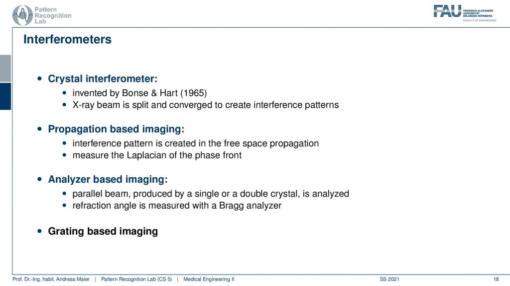
So this is the guide that we want to look at. The main reason why we want to look at it is that we can use simply a medical grate X-ray source and we can construct it with very very similar means as we already encountered in the previous videos. For the others, we typically need better X-ray sources. So for crystal interferometer, propagation-based imaging or, analyzer-based imaging, you need better X-ray sources and therefore we can’t use them typically in a lab setup. So this one you can also find the references in the textbook. We won’t use a lot of time to look into them. Actually, we just want to name them here on the slide and now we continue talking about grating-based imaging.
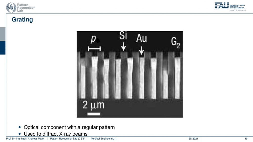
So, first of all, we need a grating and the grating has to be produced at very fine structures. You see here that we have gold and silicon layers and the distance between two subsequent layers is two micrometers. So that’s a very fine structured grating and this grating can then actually be used to create these interference patterns. Now a key problem with this is that it is typically constructed using a silicon waiver and a problem that we have is that the silicon waiver has a diameter of approximately 15 centimeters and with the 15 centimeters we essentially have a circle. So if we want to have a grating that is broad then we essentially can only have certain sizes. If we want to have very long gratings then they cannot be very broad. So this is a limitation that is caused by the manufacturing process. If you can manufacture them, you can then go ahead and build a grating-based interferometer.
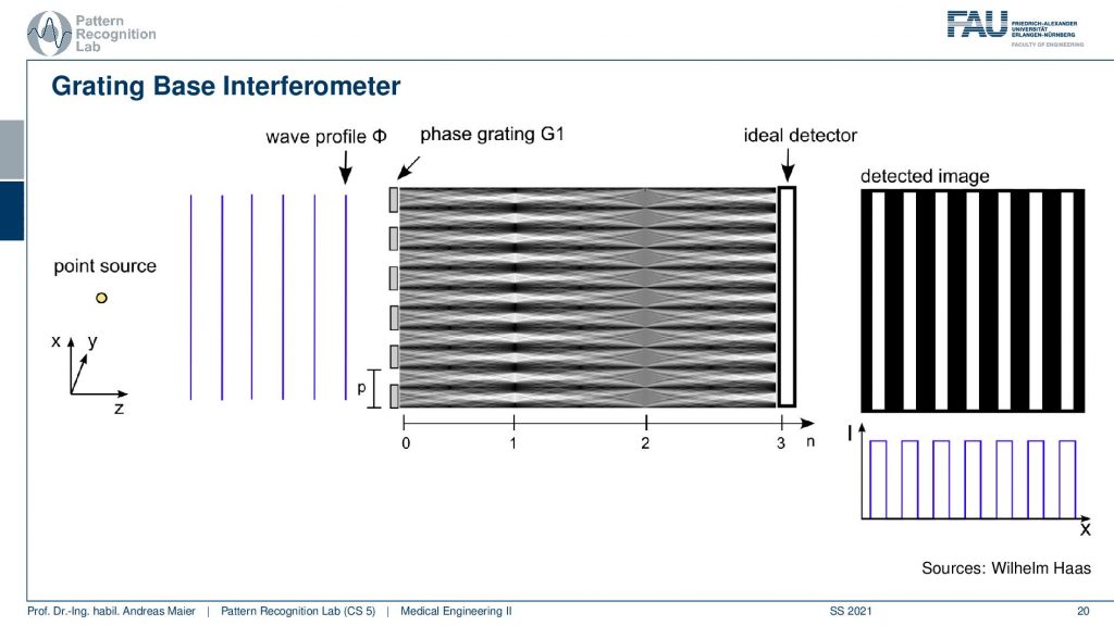
So this is what you would like to do. You would like to have a point source that creates this uniform wavefront. And then you need a phase grating the G1 and this constructs then our interference pattern. Then you go into the right type or distance you use an ideal detector and there you go you get the french pattern.
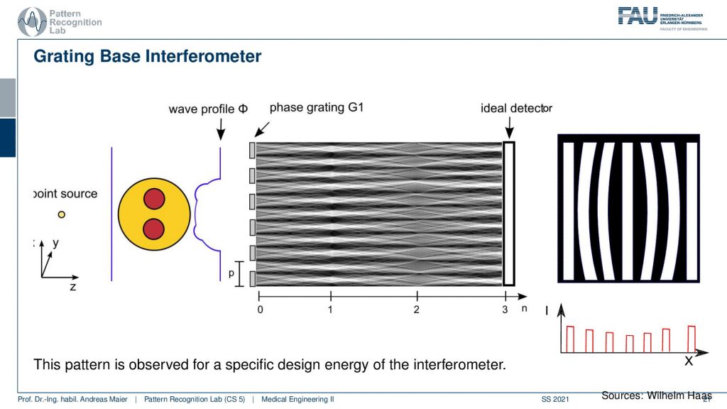
Now, what would happen if we place an object here. So we place an object. We have the grating here and then the detector here. What we would observe is a change in the fringe pattern. So the object causes the fringes to shift and also to change the magnitude. So you can see that here there’s also a change in the magnitude of the fringes and they shift. We can use this effect in order to measure the information that we would like to have.
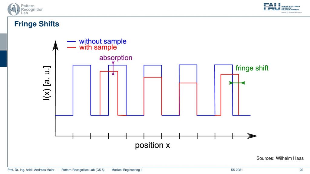
So in this case we would now have the signal without sample and with sample and this allows us to determine the absorption because that’s the difference in terms of the magnitude of the two signals. Then there is the shift of the fringes that gives us the differential phase. So this is exactly what you would like to have sounded great. So let’s just build it and then you build the system.
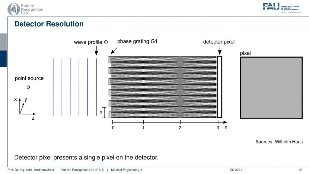
The first thing you realize is you put your detector pixel here and all you measure is gray because our pixel they’re this huge. This is one pixel. Now our interference pattern has this frequency here. So all is average out to this gray kind of color here and we can’t measure it because our detectors are way too big to measure it. So are we doomed? Well, let’s think about this again. Maybe we can use a trick.
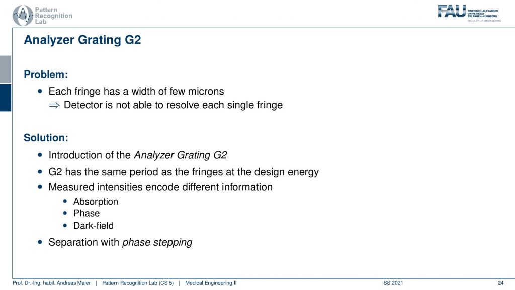
So the problem here is that the fringe has a width of a few microns. So we can’t see it on the detector pixel because the detector pixel is maybe 50 microns or, 150 microns. So it’s way bigger than the actual fringe pattern and this is why we introduce the Analyzer Grating G2 which has exactly the period as we would expect in the fringe pattern. So the fringe size is determined by the design energy and G2 is constructed exactly in the way that it has the period of our expected fringe pattern. If we have that then, we are suddenly able to measure the absorption phase and dark field. So that’s cool! The measurement procedure is called phase stepping. Why is it called phase stepping?
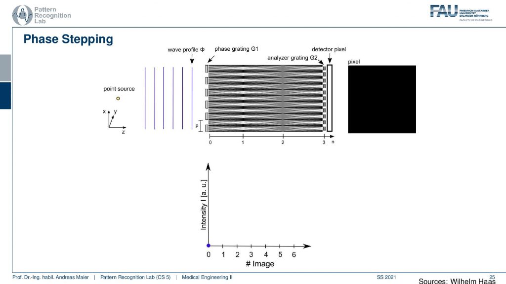
Well because we have to step. Now we have a measurement, our point source, wavefront. Here we have our fringes and here we have the right type of distance and here is our detector pixel but now we put it in the analyzer. Grating you see the analyzer rating here and this analyzer. Grating is now positioned in the way that it’s exactly facing the white fringes. So all of the white fringes are blocked at present and we can’t see them and as a result, everything on our pixel is black. So our observed value over the entire pixel is zero. Note that we have some arbitrary units here but let’s just say it’s zero. So this is the result of the measurement.
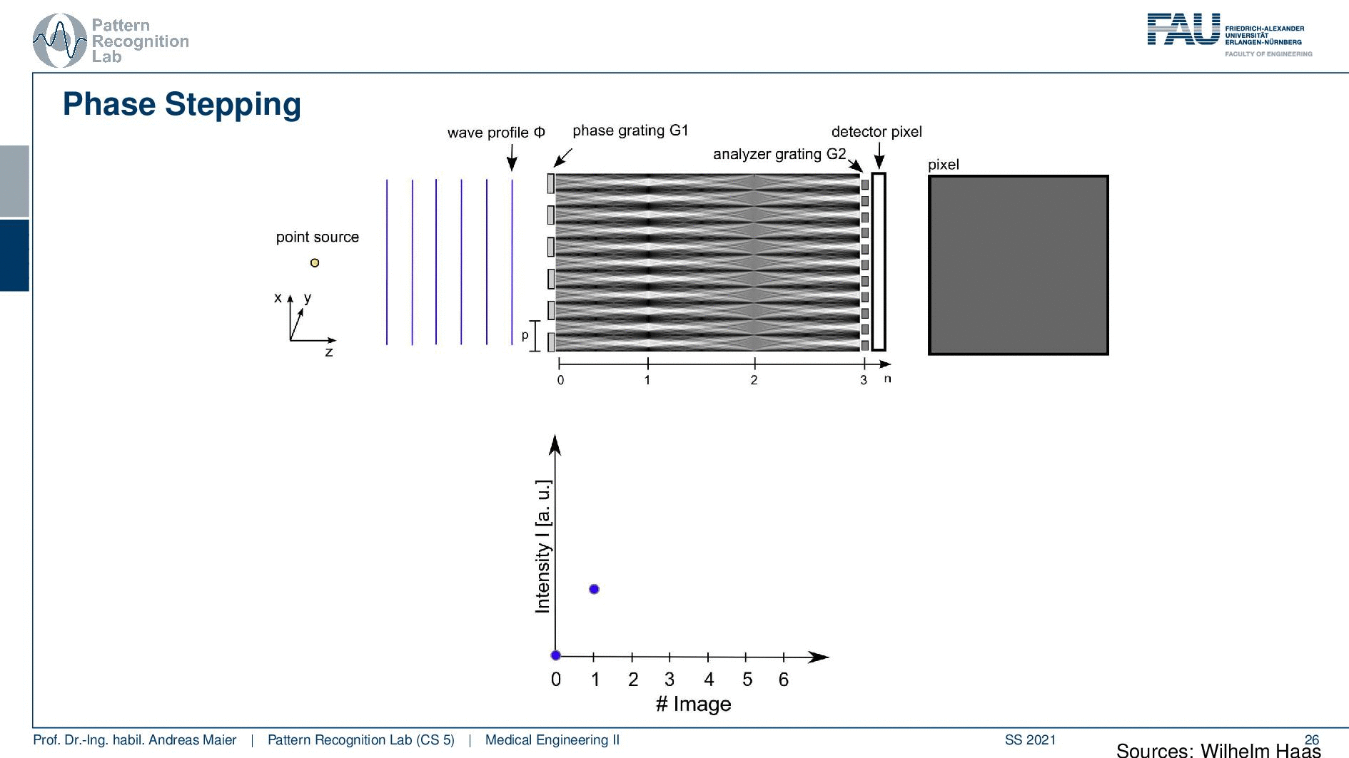
Now we shift our pattern slightly and if we shift it slightly we start getting some signal because we gradually move from the white fringe to the black fringe and we get some signal. We just did a small step, but we can reconstruct already some signal in the pixel. Well then we can step one more step and another step and you see how it gradually becomes white. So now we have a maximum here and we can now determine essentially the magnitude of the average magnitude of the bright fringes. Of course, we can then step ahead and you see that then the pixel gets dark again because we are moving with the period again over the bright fringes and everything disappears. So this is how we can construct essentially this kind of triangular shape and these triangular shapes are a surrogate measurement for our wavefront.
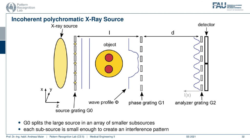
So from these triangular shapes, we can now essentially measure our phase-contrast the absorption and the dark field. One problem that we didn’t talk about is that we also have medical grate X-ray sources and they’re as large as our detector pixels. Well at least in the schematic but they are approximately in the same ballpark and much larger than the actual fringe patterns that we want to produce. But here we can use this trick again of using essentially many slits. So we introduce this grating G0. With the grating G0, I’m able to produce even from a medical grate X-ray source a uniform propagation pattern. Then I place my object. This distorts the wavefront in a way then I go to my phase grating that creates the fringe pattern and in the right distance, I’m measuring here with my detector. I move the analyzer grating and this allows us to get all the information that we need for phase-contrast and dark-field imaging.
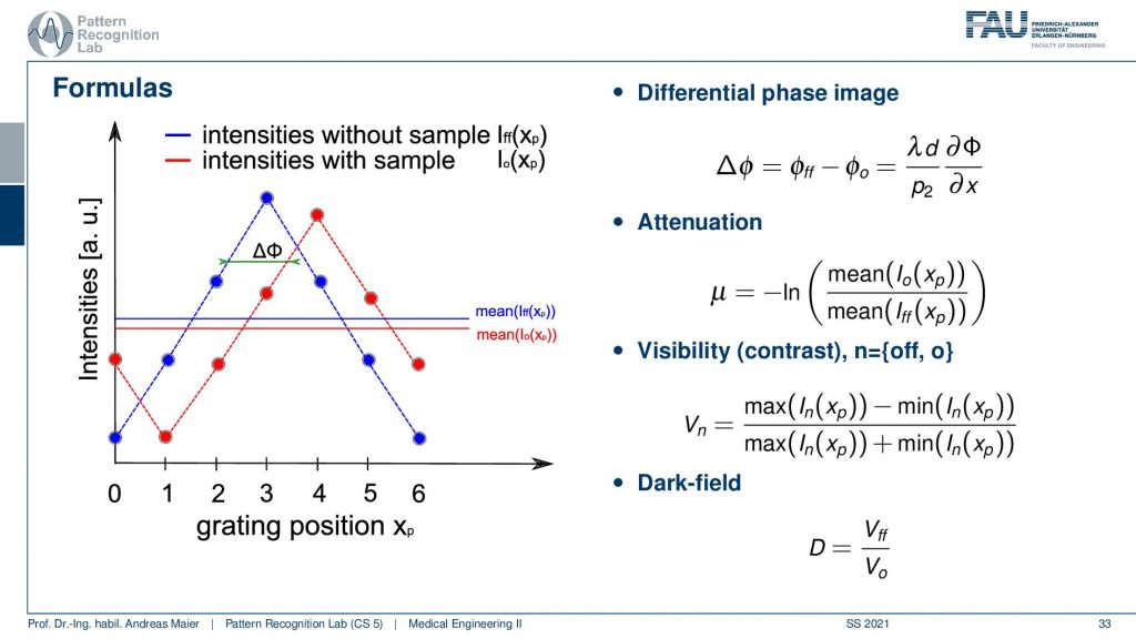
So if we do so then we get essentially these triangular waves and from those, we can now measure without sample and with the sample. This allows us to reconstruct the phase here. This is how we see the phase. We can take the means of the two waves and essentially compute the fraction of the two and this gives us the attenuation. We can also compute something that is called visibility. So this is essentially the maximum and the minimum subtracted divided by the maximum plus the minimum. This we can compute for essentially the configuration with and without object and then we take the two and compute the fraction and this gives us the dark-field signal. So you see we have this complicated measurement setup but we get essentially a surrogate signal of the waves and actually, this describes the average behavior of the waves in that pixel and from that, we can reconstruct the desired information. So that’s cool and that was all the information that we wanted to have.
Let’s spend a couple of words on darkfield imaging.
So the darkfield imaging which is the last value that we computed is caused by ultra small angle scattering.
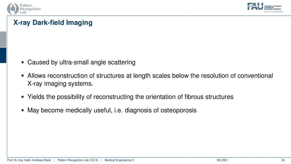
An ultra small-angle scattering is introduced by structures. So we can visualize essentially very small scale structures that lie way beyond the resolution of the imaging system. So we see micrometer structure effects in pixels that are 50 or 100 micrometer large. So it’s an order of magnitude different, but we can still measure the effect this way. This is cool and what’s also cool is that it’s dependent on the orientation. So we can also figure out the orientation of fibers because if I look along with the fiber, there is essentially no micro angle scattering. But if I look perpendicular to the fiber I get scattering here. This means that depending on the orientation of the fiber i get a different scattering signal. This then allows us to reconstruct the actual orientation of the fiber and we think that this information may be very relevant for osteoporosis or, other kinds of applications where you’re interested in the configuration of fibers. So that’s pretty cool!
Let’s look into a couple of examples.
This is an example here by Franz Pfeiffer from TU Munich.
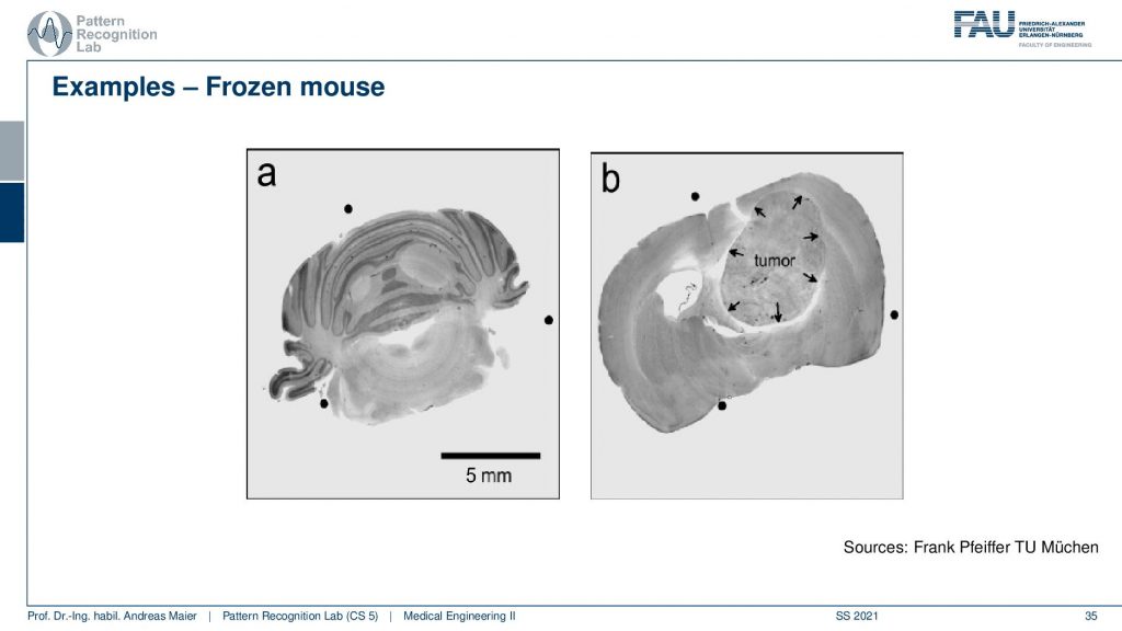
This is an example of a frozen mouse and here you can very clearly see a tumor for example.
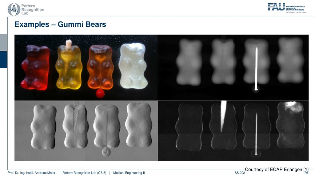
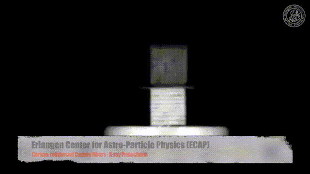
Another example here is from the Erlangen Center for Astro Particle Physics and there they did an experiment where they looked at gummy bears. So you see we have four gummy bears here. They appear to be just regular gummy bears but actually, there were a couple of modifications to them. So this guy here actually has been impaled with a toothpick. Then the third gummy bear here has also been pinned down with a regular pin. Then we have the last guy this is the white gummy bear and the white gummy bear just looks like a regular gummy bear. So let’s see what happens in the absorption image. The first gummy bear is just fine second coming there seems to be fine. For the third gummy bear, I see the needle. So this is a metal needle i see it. In the fourth gummy bear, there is nothing to see. Let’s look at the phase-contrast image. In the face contrast image, we see this guy just regular. Something is going on here in the phase contrast image here in the 2nd and 3rd gummy bear. So in the phase-contrast, we see a little more. The 4th gummy bear only appears very regular. Well, let’s look at the dark field image, and in the darkfield image, you see what’s happening. So first of all our toothpick has wooden fibers and they scatter they have this micro-angle scattering. So there’s a huge signal here. The pin is also visible. The pin doesn’t do a lot of micro-angle scattering. But it causes beam hardening and the beam hardening also causes a certain effect that it’s visible in the darkfield image. And lastly, we see this guy up here. I’m not sure if you have noticed that but actually, the guys from ECAP inserted some small beads into the gummy bear and they cause scattering. So we can see how these microstructure beads and produce a dark-field signal that you can’t see in any of the other imaging modalities. So it’s just not present but we can see it in the dark field. Such small microstructures may be a game-changer for the discovery of breast cancer onset. Because we think it’s associated with micro-calcifications and this could be a relevant technology to diagnose breast cancer early. Well, what else?
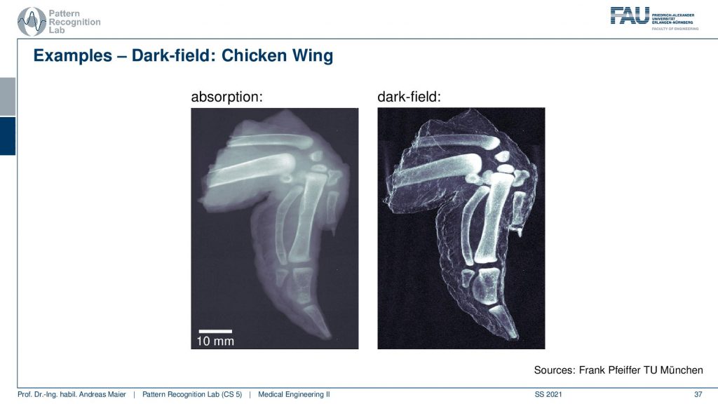
There’s also the idea about osteoporosis. This is the absorption image. This is the darkfield image. You can see that we get very high signals here and there is the belief that it might be related that the small holes in which the cells the osteoblasts live. When they stop producing additional bone material, these holes get bigger and they may introduce the scattering here. But then again you know the bonds are also very dense here and we are not exactly sure but this could also be related to beam hardening. So we see some signal, but we are not entirely convinced that this is a game-changer for osteoporosis. Well, what else can be done?
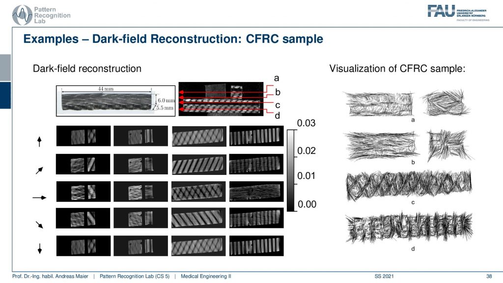
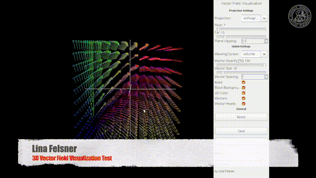
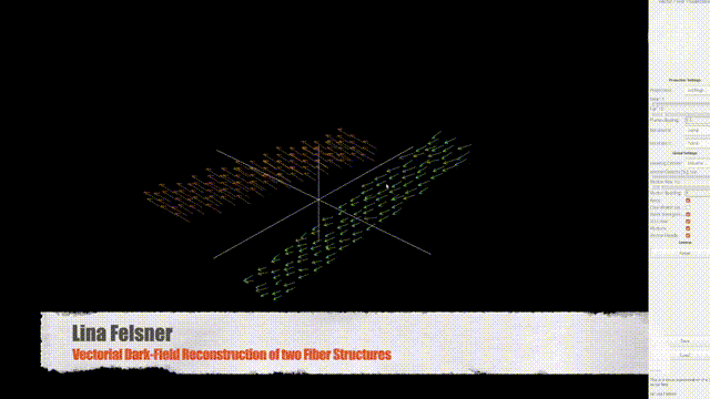
We’ve seen that we can reconstruct actually fiber orientations and this is actually a work of our lab and the experimental physics here in Erlangen together. So we were able to reconstruct the orientation of the fibers in a voxel. You see here this is the piece that we looked at. So these are reinforced carbon fibers and they’re aligned essentially in a way that you have carbon fibers on top of each other and in every layer they have a different direction. So if you image them and then look at different slices, then you can resolve them also here. You see that in every slice you have a different orientation. So this is the projection in certain directions. So in these images, we only show scalar components. So we essentially compute the inner product of these directions with the actual voxels and then you get images like this. This is difficult to follow and this is also why we then used the vectorial information. We started tracking particles that are essentially propagating along with the vector directions. If you do that then you can create images like this one and they very clearly show that in different slices you have a very different orientation of the fibers. Again the fibers are smaller than what we actually can reconstruct. So we can reconstruct fiber orientations on average per voxel that is below the resolution of the actual reconstruction grid. So that’s pretty cool! I have one more sample here.
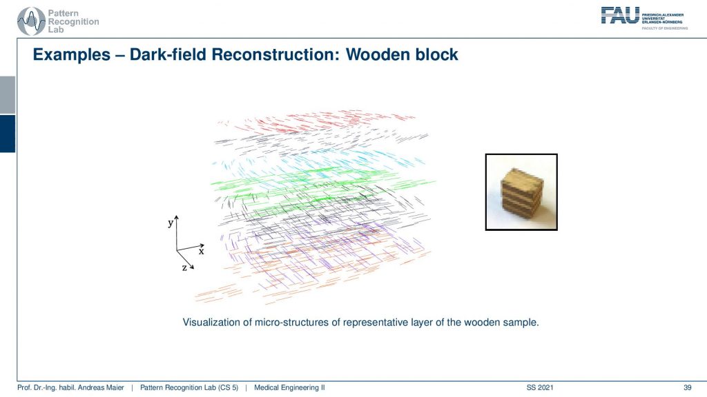
So this is a woodblock. It also has fibers in different orientations and here we reconstructed them and show them and you can very clearly see that they have different orientations in the different layers. So also a very nice result. How can this be measured?
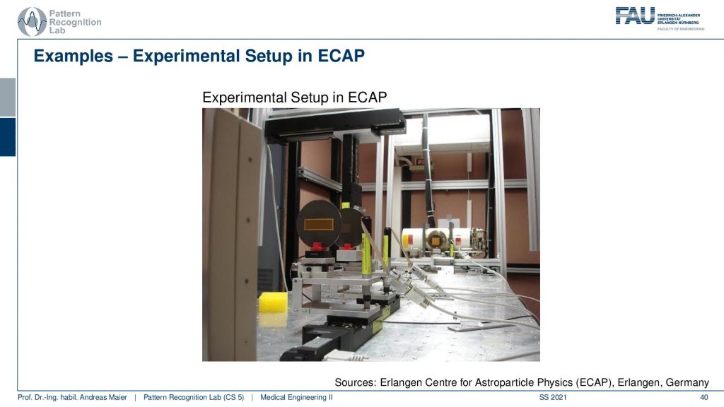
This is the actual measurement setup in the Erlangen Center for Astroparticle physics here in Germany. Let me point out a couple of things here. This is a medical grate X-ray tube. This is the G0. So this is where the coherent source is being generated and then you have the phase grating. So this is the G1. You would probably place your object somewhere here and you have the detector with the face stepping actually in this position. Now you see the long distances here but they have to be aligned in micrometer ranges. So you have to be very careful in the alignment and obviously, you have to spend quite a bit of time in order to have the optimal alignment done for all of these gratings. Also, this may be dependent on temperature, because it’s micrometers and if you have a temperature change then also the gratings may shift slightly and so on. So this has to be recalibrated quite frequently and you do that best with automated means.
This brings us already to the end of this video. I highly recommend the book chapter by Johannes Bopp.
He actually summarized all of this in this presentation as well as some additional references. So please have a look at our textbook and this already brings us to the end of this video.
So you’ve seen now a very experimental kind of imaging modality where we are essentially still constructing the actual imaging techniques. Still, we’ve seen that it may have a couple of advantages. So it would actually be great to see whether this actually translates into clinical practice or not. You see of course the reason why it’s not yet translated to clinical practice is that we have to provide proven evidence that it will improve the actual clinical practice. So this could not be demonstrated yet, but at the point where we can show that it makes a difference for the treatment of the patients. I’m very sure that this kind of technology will translate very quickly into the clinic. So this is the kind of fundamental trade-off between fundamental research, developing new imaging modalities and new face contrasts and image contrasts, and the clinical need. Obviously, the technology will only translate if there is an unmet clinical need that drives the benefit of the patient. This already brings us to the end of this small video. I hope you enjoyed it and I’m very much looking forward to seeing you in the next video when we talk about Nuclear medicine and functional imaging. Thank you very much for watching and bye-bye.
If you liked this post, you can find more essays here, more educational material on Machine Learning here, or have a look at our Deep Learning Lecture. I would also appreciate a follow on YouTube, Twitter, Facebook, or LinkedIn in case you want to be informed about more essays, videos, and research in the future. This article is released under the Creative Commons 4.0 Attribution License and can be reprinted and modified if referenced. If you are interested in generating transcripts from video lectures try AutoBlog
References
- Maier, A., Steidl, S., Christlein, V., Hornegger, J. Medical Imaging Systems – An Introductory Guide, Springer, Cham, 2018, ISBN 978-3-319-96520-8, Open Access at Springer Link
Video References
- The Double Slit Experiment Animation https://youtu.be/Kdi4e76UvO8