Emission Tomography

These are the lecture notes for FAU’s YouTube Lecture “Medical Engineering“. This is a full transcript of the lecture video & matching slides. We hope, you enjoy this as much as the videos. Of course, this transcript was created with deep learning techniques largely automatically and only minor manual modifications were performed. Try it yourself! If you spot mistakes, please let us know!

Welcome back to Medical Engineering. So today we want to talk about nuclear medicine and functional imaging and in particular, we want to see how we can use tracers to create images of the metabolism inside the body. Therefore we will have a short excursion into the basics of radiation and how radiation can also be constructed into radioactive molecules and these molecules will be used in order to create the image contrasts here. So looking forward to introducing some nuclear medicine to you guys.

Well, let’s introduce the topic of nuclear medicine.

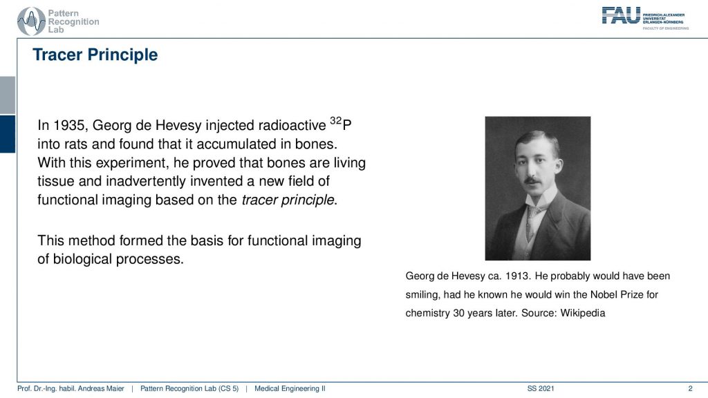
There is a very interesting question that came up in the early 1900s. So here Georg de Hevesy used radioactive tracers in order to figure out whether there is metabolism in the bones or not. So the interesting thing is up to that point in time, people weren’t sure whether the bones are just like stiff parts inside of the body or whether they are also doing any kind of metabolism. So the bones are hard and dense and it wasn’t clear whether there is something useful happening inside and this could be shown with tracers. So Georg de Hevesy injected radioactive phosphorus into rats and found that it accumulated in the bones. So with this experiment, he was the first to show that bones are actually living and that they can also saturate with something that you inject into an animal and that they accumulate in the bones. This gave rise essentially to the tracer principle. The tracer principle is that you take a radioactive isotope, put it into the metabolism, and then you measure its distribution. This is the core idea of nuclear imaging. 

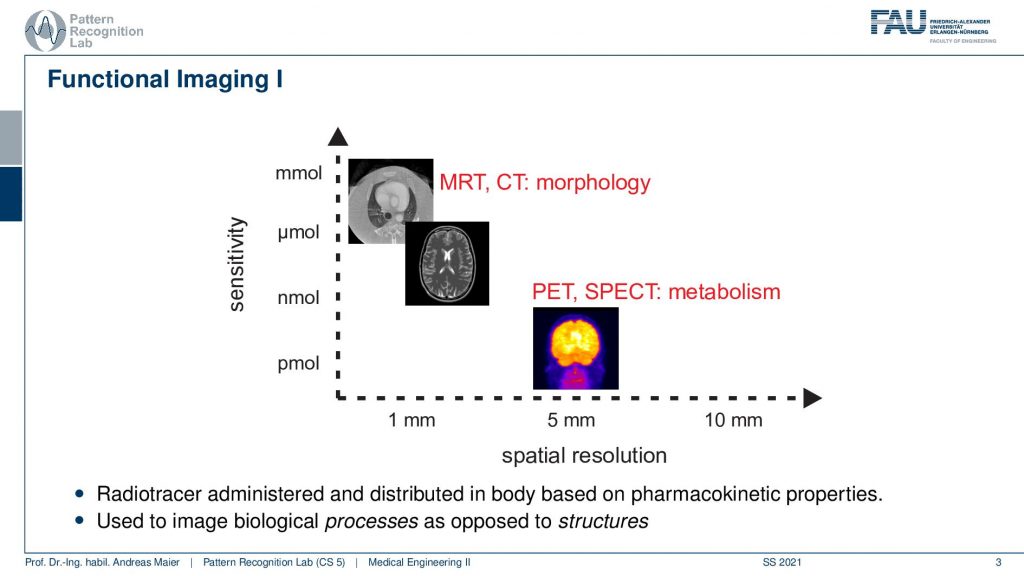
So here we are talking about functional imaging and you see that the nuclear kind of imaging devices PET and SPECT measure metabolism and they have a rather coarse spatial resolution. But they’re able to actually measure picomole. So very very fine amounts of tracer can already be measured. This is also very important because we want to be able to only use a minimum of radioactive traces inside the body because of course, this is also ionizing. It can break down the DNA strands and therefore it may also introduce cancer. So we want to be very careful with that. 

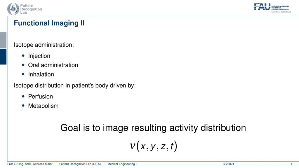
So we do that and the functional imaging is then using some isotope that is somehow inserted into the body. It can be injected. It can be swallowed. It can be breathed. So some way how to get it into the body. So it’s injectional, oral, or inhalation, and then the distribution of the isotope is somehow going into the body either by perfusion or, metabolism. The goal of nuclear imaging is to reconstruct the activity distribution of the tracer in three dimensions and in time. So we have now four-dimensional images and we want to figure out where the distribution is going and how it’s being processed inside of the body and we can use that to investigate the metabolism. 

Let’s have a look at the physical foundations.

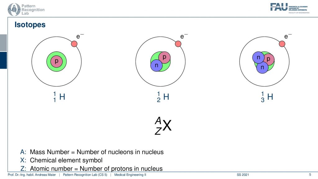
In order to understand the following. We have to look a bit into nuclear physics and in particular into isotopes. We know that the number of positrons in the actual core determines the actual element. But we can have different types of elements. So all of this is hydrogen. But you can have hydrogen with an additional neutron or with two additional neutrons. These are essentially the different variants of hydrogen and some of these isotopes are radioactive and they kind of disintegrate and by doing so they go into nuclear decay. So they cause radiation and this radiation in our case is the kind of effect that we want to use in order to figure out where the isotope is going. In order to figure out the metabolism, we just don’t use the individual isotopes but what we often do is bind them into a specific molecule and this molecule is then relevant for the actual metabolism. So for example- sugar or other molecules that are a relevant role in our body’s metabolism and then we can figure out where the isotopes are going. We can see the distribution also in a three or four-dimensional image. So that’s the key idea. 

Now there’s of course a little more to that. So first of all we have radioactive decay and there are a couple of decay mechanisms and that depends on the kind of isotope that you’re using. So there’s α or, β decay. There are electron captures. There’s isomere transition and spontaneous fission that can occur. But we are only actually interested in the ionizing radiation here.

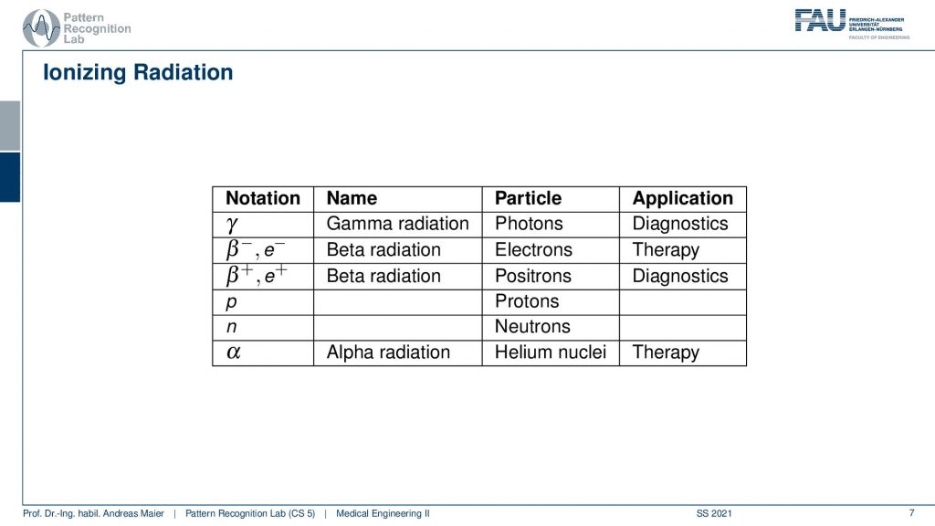
Different kinds of decays can happen. So we can have a pure γ that is produced and this is γradiation and this is essentially a photon that is emerging. Then there is also the β^– and β⁺ decay and the β⁺ is a positron and positrons are also very relevant for us because they can also be used for the tracer principle. So both of them are used for diagnostics. The β^– and also α radiation is used for therapy. So there are also therapies where you use the ionizing radiation that is caused during radioactive decay. But here we mainly focus on the diagnostic applications. This means we’re interested in γ decay and β⁺ positron decay. 

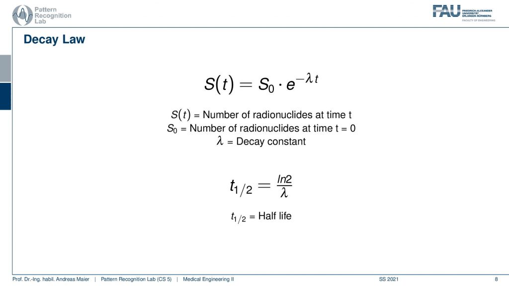
Now if you have such an isotope it will follow the Decay law. Here you see this is essentially the number of radionuclides at the initial time t=0. So this is S₀ and the number of radionuclides that still are present in the body can be determined by such an exponential decay law. Here we have λwhich is the decay constant and from λ we can compute the half-life. Half-life is essentially the time the logarithm of 2 is divided by λ. So this is the amount of time that needs to pass that you have half of the number of radionuclides still present. So how does this look then like?

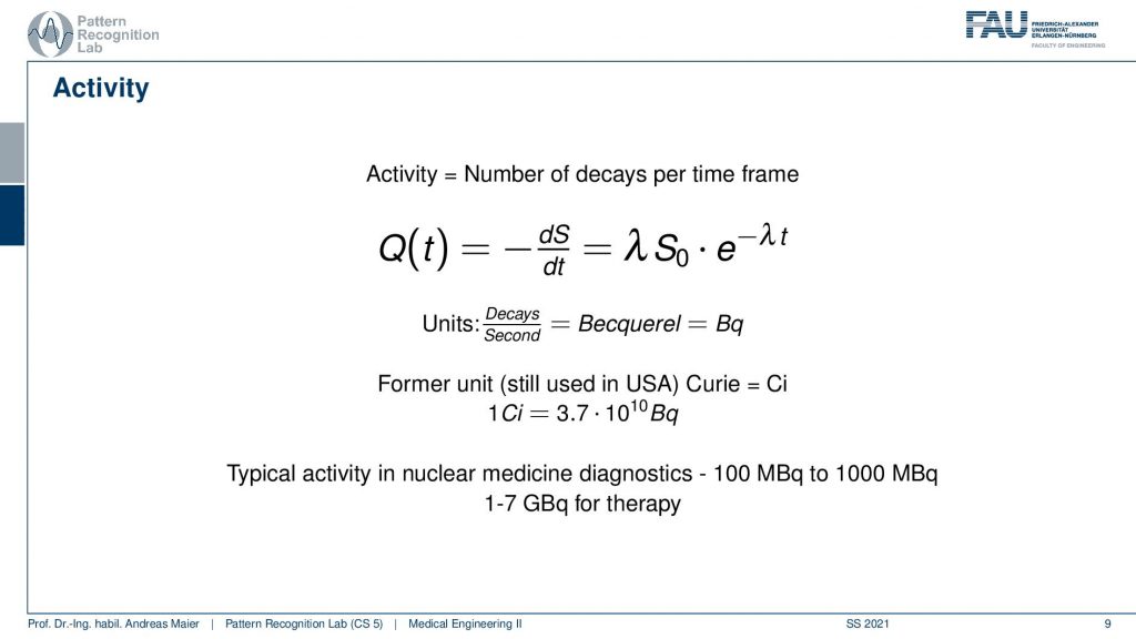
Well, actually there are a couple more things we need to talk about. One thing is Activity. Activity is the number of decays per time frame. So activity is associated but it’s essentially the derivative of the radionuclides with respect to time and you can compute the activity here with this equation and typically unity is Becquerel. Becquerel is the decays per second and this is measured in Bq. There’s also a former unit that still is used in the USA and in the USA you measure Curie and it is abbreviated with Ci and 1Ci is 3.7 times 10 to the power of 10 Bq and Becquerel is also something that you can measure with a Geiger counter. So this is a device that allows you to measure how many radioactive decays are happening in your environment. And this is exactly also what we are kind of afraid of when we are talking about nuclear power and so on. There we measure the activity of the radioactivity and in our case, we want to use the radioactivity actually to figure out how the metabolism is working inside of our patient. Typical activity in nuclear medicine is a hundred to a thousand MBq and in therapy, you have one to seven GBq. So these are the numbers. You should have this in mind when you talk about these things. 

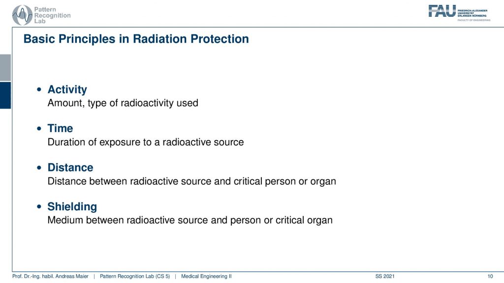
Now what’s relevant now is that we talk about the activity. This is the amount and type of radioactivity used. The time is the duration of the exposure to a radioactive source. The distance is very important because the distance between the radioactive source and the critical organ of a person is relevant because you have the inverse squared distance law. So the farther you’re apart the less the respective source is actually interacting with the tissues and then there is also shielding. So you can introduce a medium between the radioactive source and the person or the critical organ and this can also help you to prevent the radiation from going to the locations where you don’t want to have them.

So the problem statement in emission tomography is that we want to reconstruct the distribution of the activity. 

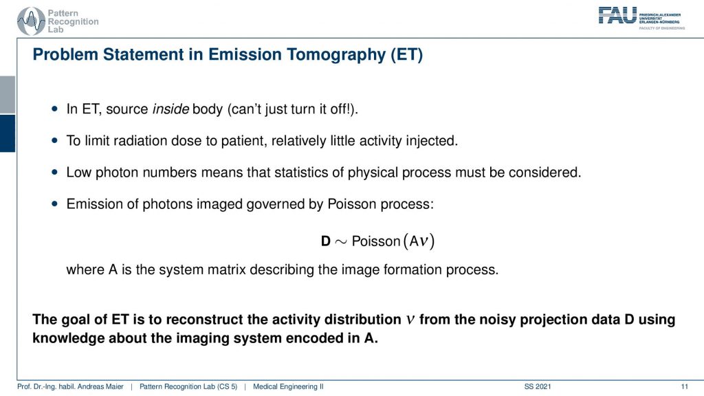
The key problem is that in emission tomography the source is inside the body and we can’t just turn it off. So in X-rays, I turn off the X-ray tube and X-rays are gone. In emission tomography, all of the activity is already inside the patient and the patient itself is irradiating the radiation. So you also have to be very careful when you move those patients after diagnostics because they irradiate the radiation themselves. So they have to stay in hospital until they are no longer radioactive. Obviously, there’s the relevant half-life and the other relevant thing is that there are also natural means how the tracer can leave the body for example through the bladder. So this is also something that you can use in order to figure out whether a patient is still radioactive or not. So to limit the radiation dose to a patient with very little or relatively little activity injected. Because we want to use it only for diagnose. So this is also where we have to work with these very little amounts of radioactivity and then reconstruct them. Technically we get very low photon numbers and this means their statistics and the physical process must be considered. So you’ve seen that the Poisson distribution is different from a Gaussian distribution with low count numbers and this will be very relevant also for this chapter. So typically the distribution that we want to reconstruct is the result of a Poisson process and this is essentially the activity from all of the voxels that contribute to our detector element. So this is how we can describe this A essentially describes how all of the voxels interact with our detector element. So again we have something like a system matrix that describes the image formation process. So the goal of emission tomography is to reconstruct the activity distribution from the noisy projection data D using knowledge about the system geometry. So this is what we want to do. 

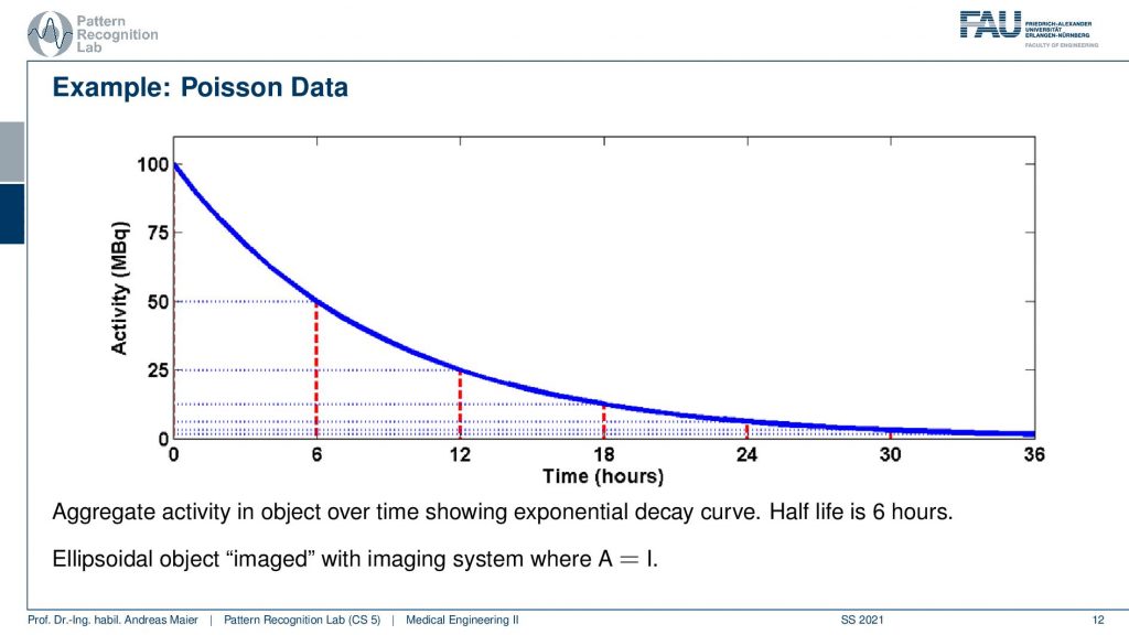
So one thing that we have to keep in mind is that our activity decays over time. Now you see that after six hours I only have half of the activity after 12 hours again half 18 hours. So we have a six-hour half-life here. So we see this exponential decay happening and this is also very relevant for the image quality.

So if I image at t=0 then I have very little noise. But if I would image let’s say six hours later or if I measure like 12 hours later you see how the noise increases. So the more I wait, the more the noise increases because that is dependent on the activity and the half-life that is used in this exponential process. So the image noise increases notably here in this case and this is also something we have to keep in mind. 

Now let’s talk a bit about image formation. 

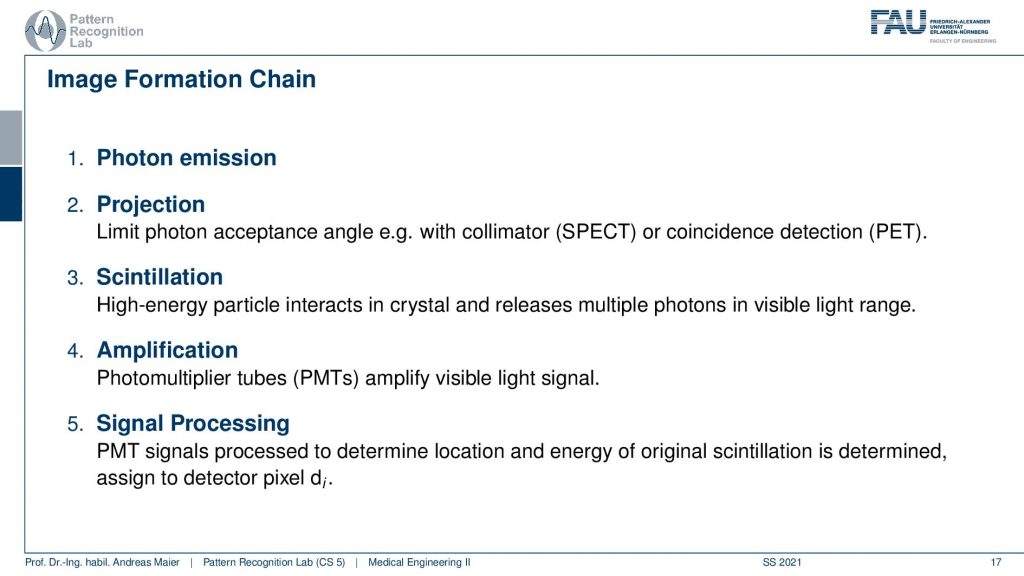
So first of all, we have to somehow get photons that we measure. Then the photons are projected somehow onto a detector. Then we use some tricks to figure out which of the photons are the relevant ones. This is called scintillation. Then we amplify, this is done with photomultiplier tubes PMTs. Then we get essentially a light signal and finally we do some signal processing to get the reconstructed image. So this is the main outline of the image formation chain. 

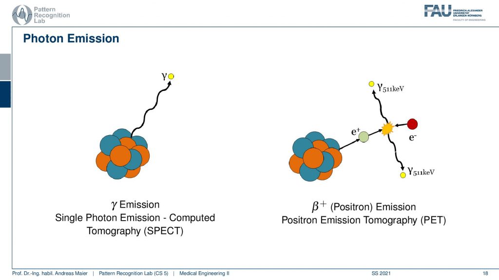
Now if we want to do that we have to start with the actual photon emission and there are two effects. We have seen that there is the γ emission. So this is already producing some radiation and there’s radioactive decay and then the photon goes into an arbitrary direction. This is called Single Photon Emission Computed Tomography (SPECT). There’s another kind of radiation source that we can use. This is the β⁺ decay (positron) and this leads then to Positron Emission Tomography (PET). The key difference between the two is that in PET we have a Positron that interacts with an electron and they annihilate. They just disappear but they don’t disappear without a trace. They actually create two γ and these γ quanta are flying out in opposite directions and both of them have exactly 511 keV. So you get two γ quanta that are exactly emitted into opposing directions and this is nice because this forms a line. So in PET, we can use the coincidence detection to figure out which of the two γ quanta actually are from the same event. If we figure out that this is the same event, we can get the line that connects the two quanta. Then from the joint attenuation, I can figure out how much attenuation was applied on this line. So this is nice and this gives us some advantages for PET reconstruction because we have some advantages in terms of knowledge about geometry. 

Now let’s go ahead and put this to use. 

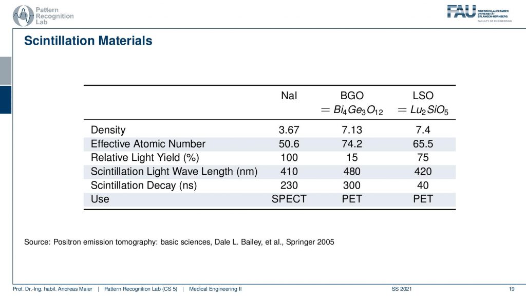
So one thing that we now have to do is we have to scintillate. So we somehow have to produce a measurable signal from our γ quanta. It doesn’t matter whether it’s now PET or SPECT. We somehow have to measure the γ contour and this is done with scintillation material and there is a typical number of scintillators. So there’s Sodium Iodine, BGO which is bismuth germanium oxide and there is LSO which is lutetium silicone oxide. So these kinds of scintillators are very common. They differ by density. So you see the last two are similar in density. They differ by effective atomic number. They also have a different light yield and then they are also used essentially in different imaging systems. So in SPECT, you typically have the sodium iodine scintillators and these two here are mostly used in PET. So there you see already the difference in the construction of the system. So you need different detectors and different scintillators depending on the kind of radiation that you have so already. There we have differences. Now let’s talk about a SPECT detector.

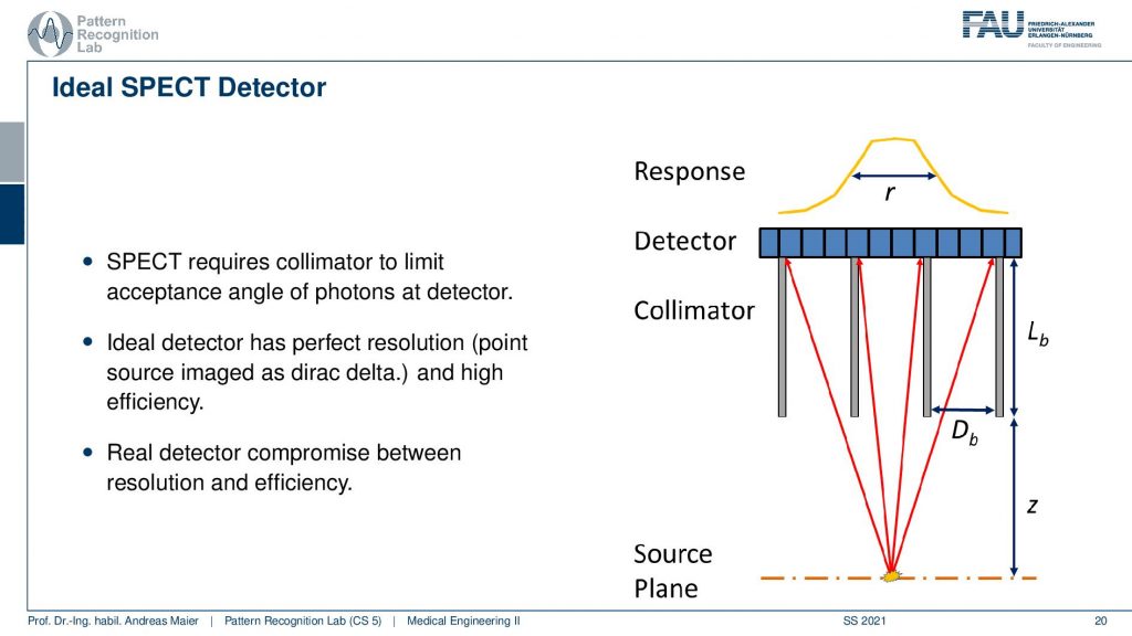
So here, we have the huge problem that we don’t know where the γ quantity is originating from. And we see that we use here something that is called a collimator. It has a very similar idea to the anti-scatter grid that we’ve seen in X-rays. So if I have some event that originates from here, then you can see that essentially if I connect it directly here, I will get a high response. But if I’m essentially going into other directions the collimator is able to block a lot of the radiation that doesn’t hit directly the detector. So here these photons all get absorbed and this then results in a point spread function that is a little sharper than if we are not using a collimator. So this essentially is a technique that helps us in building better point spread functions on the detector in particular for the case of SPECT. 

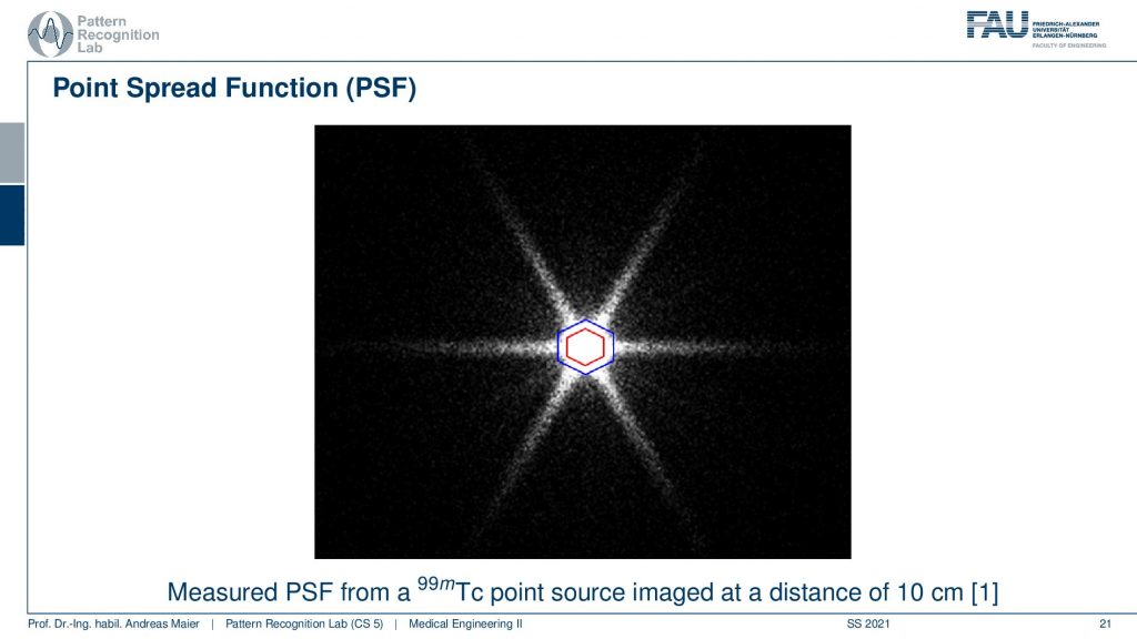
Now if we want to use that we can essentially measure a point spread function and here you see a hexagonal collimator design. You see that most of the point spread function is here but we still get these kinds of leaves and this is exactly perpendicular to the collimator blades that have been constructed. So here you see the design. 

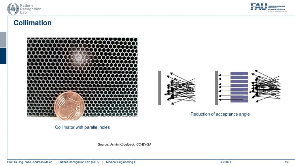
This is a collimator with parallel holes. So the holes are just not narrowing down and here you can see the schematic. So you see all of the different scattering events coming in here and only the ones that are actually in the orientation of our parallel collimator holes will be detected in the end. This allows us to differentiate all of these scattering events and we are only seeing things that come from a particular direction and of course, this is key to enable the actual reconstruction. So here you see this is a one-cent coin and this is the size of the collimator grid that is constructed. 

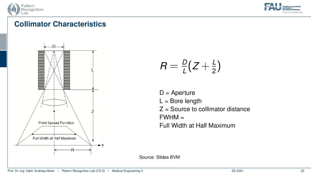
Now if we look a bit more into the characteristics we see that there is essentially a trait of with the diameter of the hole, the length of the collimator blades, and then the distance into the scene. All of this allows us to determine essentially a point spread function and we measure the sharpness of this point spread function by the full width at half maximum. So this allows us to give us the properties of a specific point spread function. Here you can see that we are able to compute a certain R. So r is essentially the distance of the slope here and R is determined as D over L times Z plus L over 2. So D is the aperture L is the ball length and Z is the source to collimate the distance. This way we can determine all of these parameters here.

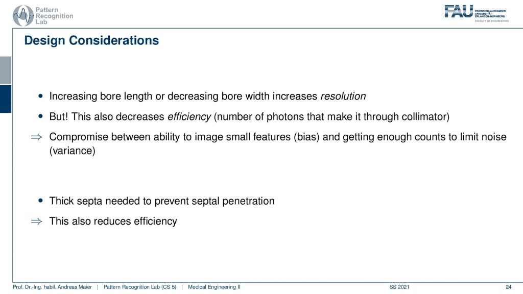
This gives us a kind of path where we can design collimators. So increasing the ball length or, decreasing the bore increases its resolution but it also decreases the efficiency which means the number of photons that make it through the collimator. So we somehow have to have a design compromise when you’re building these collimators. Then also we can build thicker scepter or, blades and the thick blades of course cause the different holes to be separated better but they also reduce the efficiency because they also reduce the area of the individual holes. So if I have very thick septa then I also have fewer photons that get detected at the detector. 

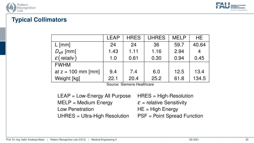
This then brings us to a couple of configurations and they don’t want to run all of this but then there are different applications and they come up with different configurations here. Depending on the configuration here, I have a different weight. You can see that the collimator can weigh between 22.1 kilograms up to 134 kilograms. So this is the high energy collimator here and then there is the low energy all-purpose collimator here and there’s also ultra-high-resolution kind of collimators and you can see configurations from them here. 

Very well. So this is the idea of the collimator and now after the collimator, I need to detect something.

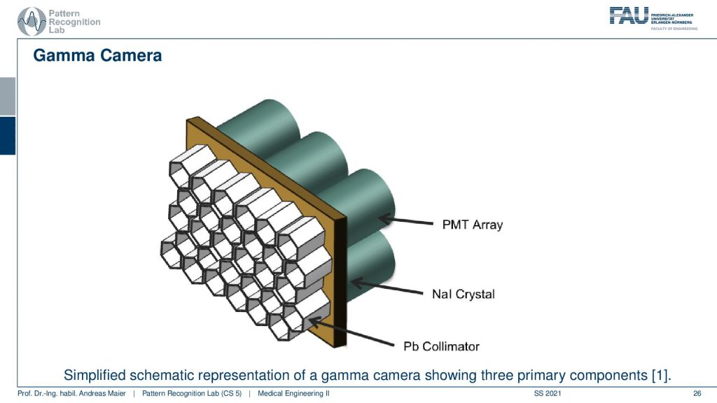
This is done with this photomultiplier tube array and we essentially have a Pb collimator. Then we have our scintillator that kind of produces the visible light and then we need this array in order to construct the actual detector and this leads to the following setup. 

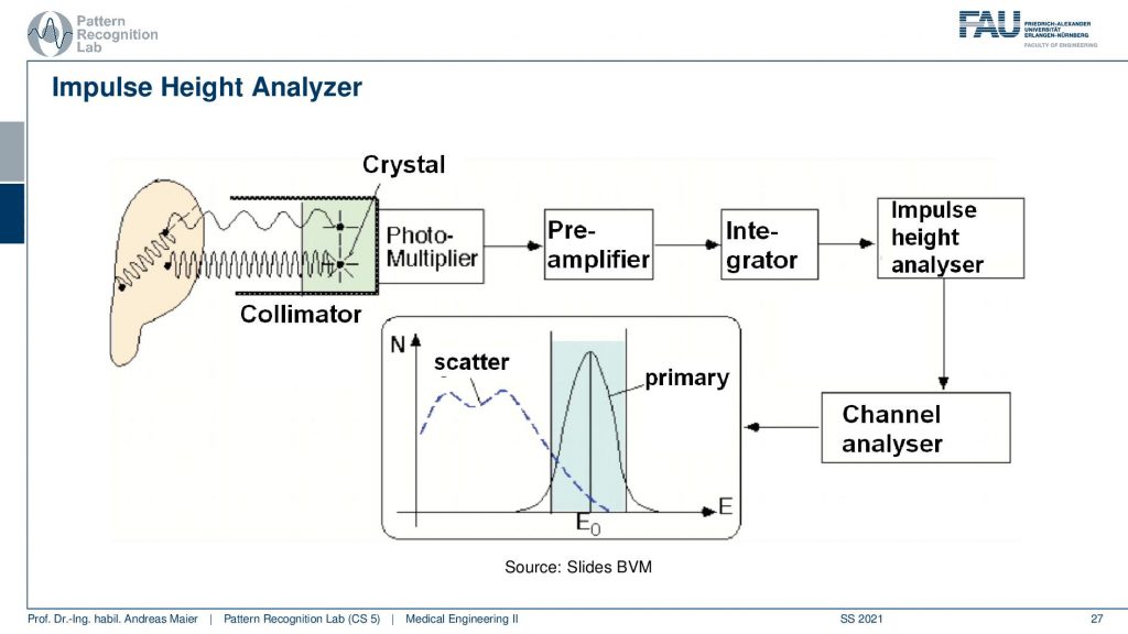
So you have some event that goes here into the crystal and this is then running through the photomultiplier. This goes to a pre-amplifier, an integrator, an impulse height analyzer, and a channel analyzer. We then get a photon count and this is energy resolved. So that’s pretty cool that in the PMT detectors we really get the spectrum. Now we can use actually the spectral information here that events that are in this energy range are primary and all of the events that are here in this energy range are scatter. So scatter correction in SPECT is very easy because I can just say okay if it’s below this threshold it’s scattered if it’s beyond this threshold it must be primary radiation because it has higher energy. So this is pretty cool and because we essentially detect the individual events, we have very few photons. We can analyze them well and use that immediately for scatter correction and getting rid of scattered signals. So this is an additional scatter prevention that we can use on top of the thick scepter. So this then brings us to the first image formation process.

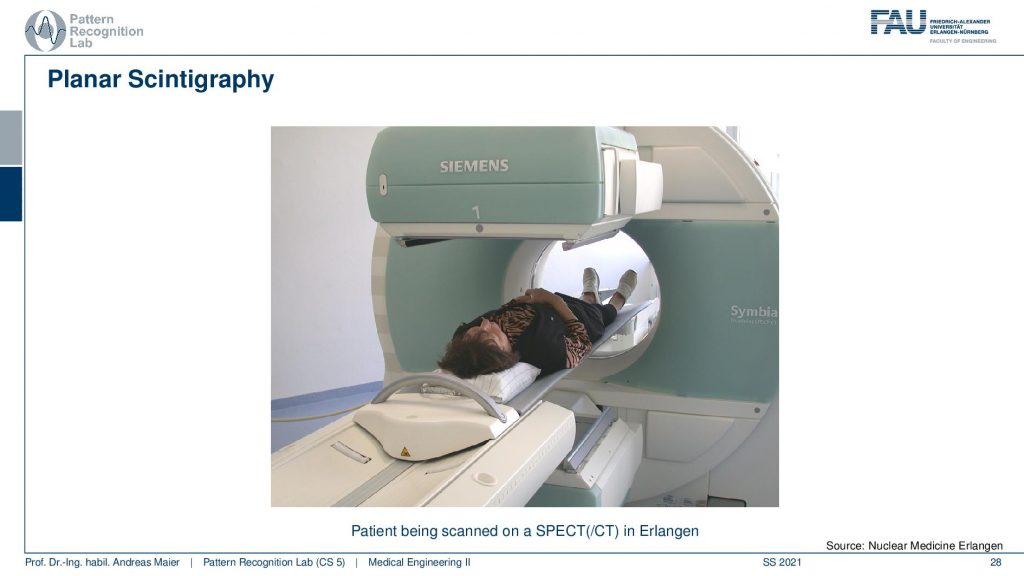
So here you see the detector and the collimator and then you have a patient here. The patient irradiates into our detector and here the images are being made. 

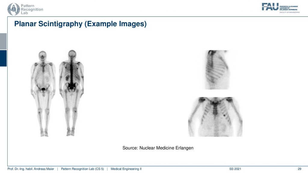
If you see then the images that you can get out of this are this planar scintigraphy. Typically we take two of these detectors and then we move along the patient. You can see because of the absorption inside of the body, there is a front and a back image. So the front and back image is different because the body itself also absorbs some of the radiation and the two detectors measure two different signals. Here you see then that you can also measure from the side or you can also measure from the front. 

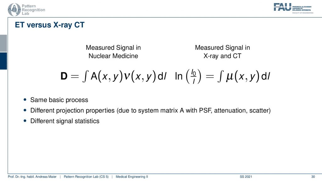
So what’s the difference between emission tomography and CT? Well, there’s a little bit of difference because you have essentially no X-ray source but you have the event emitted somewhere inside the body. So you have some kind of activity that is distributed in only a slice here but it could also be a volume. Then you have the contribution of this activity summed up and this gives the projection. So in terms of the kind of math, it’s similar because it’s the same basic process but of course, we have to know from which directions the actual contributions are. Because if everything is just contributing then just everything is connected with everything and we can’t solve. So we need to use a collimator in order to bring up a proper kind of system matrix and with this, we can then reconstruct the activity. In contrast in a CT system, you always get complete line integrals and these are completely measured. So here we always observe everything that is integrated along this line. So it has different projection properties and this results in a different system matrix and a different point spread function and obviously, the signal statistics are different. But other than that the reconstruction is to some degree similar. 

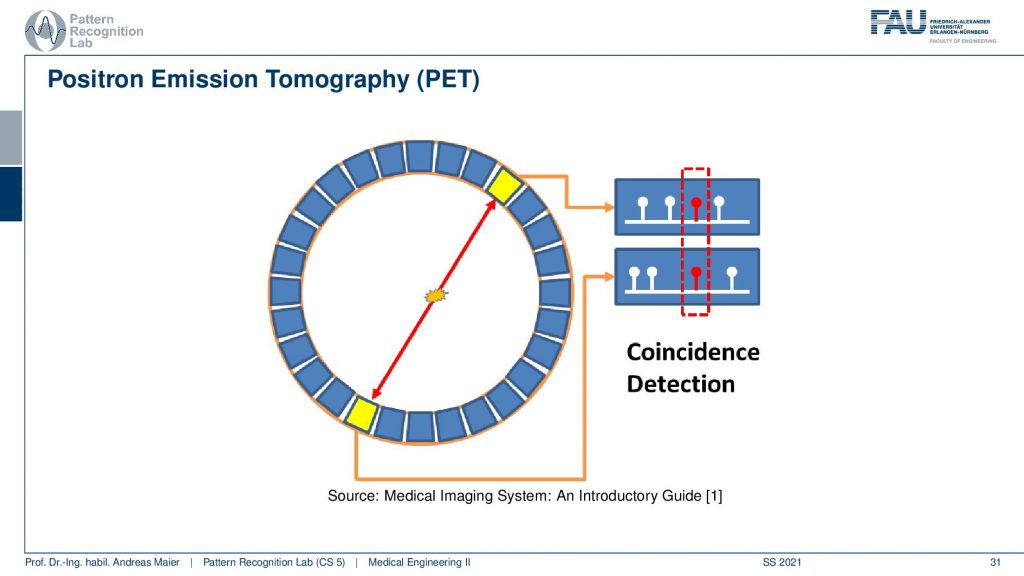
So let’s look a bit into the geometry of PET and in PET you have this event then you have the two γ quanta that are fired out. Then they get detected in the ring shape detector here and here. Then you have a very fast kind of electronics and this electronic is detecting coincident events and if you have a coincident event then you know that this ray has been used for this particular decay and that you can associate this particular measurement to this geometry here. So we can kind of get a list of events and the list of events is associated with the particular geometry in our PET system. 

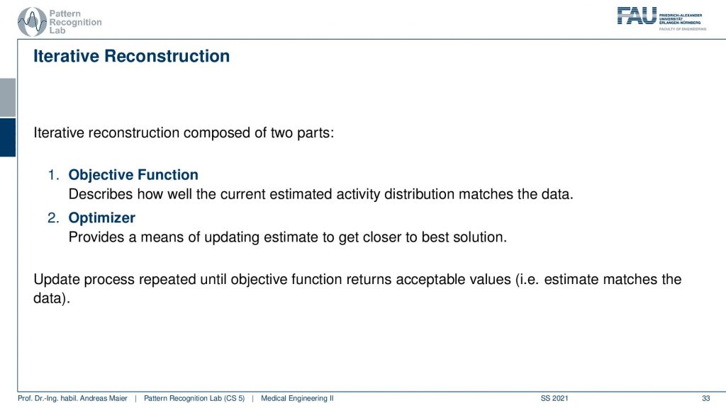
Then we need to reconstruct somehow. We do it similarly as we’ve observed before we do an objective function and then we optimize it. So we somehow described the mismatch between the current estimation of the activity and volume and what we measured. And if we’re able to describe the mismatch then we can optimize the activation in our model such that it matches the actual observations. This is the reconstruction that is done here and this is a classical iterative reconstruction approach. 

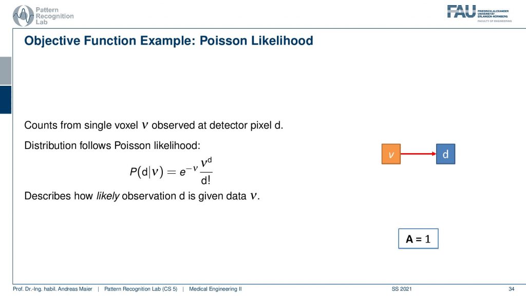
So what we need to do is we need to describe somehow how the activity and volume and the detector are associated. If I had only a single volume element and a single detector the system matrix would simply be an element with a one. So we would directly observe the activity as it’s happening in our volume. Unfortunately, that’s not entirely true but instead, we have some kind of geometry. 

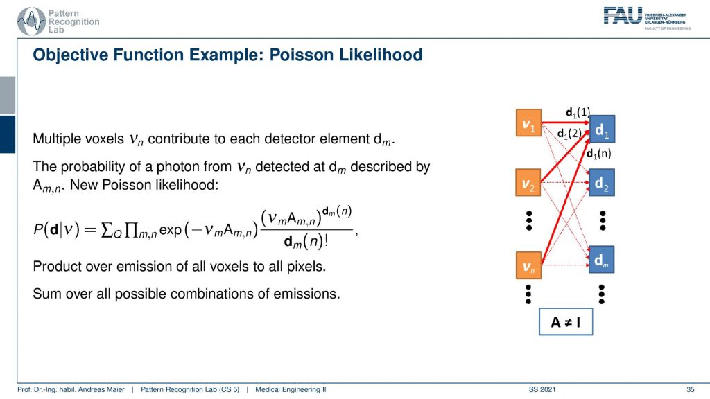
This makes it a little more complicated. Because all of the voxel elements somehow contribute to the respective detector elements and so on. So they are interconnected and the geometry now governs the configuration of the system matrix. If I use for example a parallel kind of collimator in SPECT then this essentially drives this kind of system matrix. If I have the different rays connecting each other in a PET system then this drives again the system matrix here. To describe the image formation we can express this essentially as a probability of observing the current reading at the detector given the current estimate of the activity distribution. This can then be written up as this term here. So you see that we have the Poisson distribution in here. Then a product over all the elements and in the end a sum of a Q and this gives us essentially the model that we can then link to each other and then we do a maximum likelihood reconstruction. So we seek to optimize the likelihood of this term and we do that with respect to the current activity. So this then yields an iterative procedure that allows us to update the respective volume such that we get an activity that explains best the actual observations that we got from the detector. This is nice because we can put directly the statistics into this model and the Poisson model and so on. 

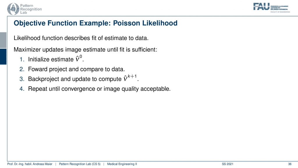
So if we want to construct then the objective function we then have to set up the previous equation. We initialize with some estimates, we project this estimate to the detector using our model. Then we compute essentially the difference by computing the fraction of the two and back project this to update our activity and we repeat all of this until we get an acceptable image quality. So this is approximately how the iterative image reconstruction in Emission Tomography works. 

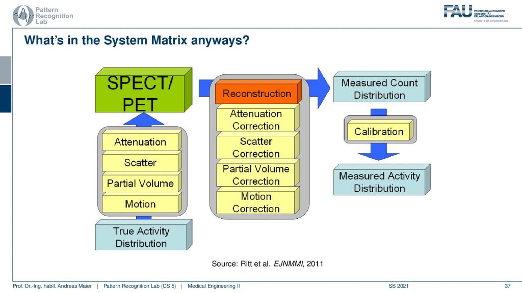
It’s a little bit more complicated because we have these many different things that take part in the image formation. So if you have the true activity distribution, there is the scans take quite a long time. So there’s motion on top, there’s the partial volume effect. There’s scattering happening and then there is the attenuation of the tissues that are actually in the patient that also causes signal loss and this is the actual observation. So if we want to reconstruct the entire thing we step by step correct for the attenuation differences, we remove the scatterer, we do a partial volume correction, and then we do a motion correction and this then gives us a measured count distribution in terms of a volume. If you can calibrate this let’s say there is a source of known activity in the field of view. Then you can get a measured activity distribution. So then you have a calibrated quantitative kind of scanning procedure. 

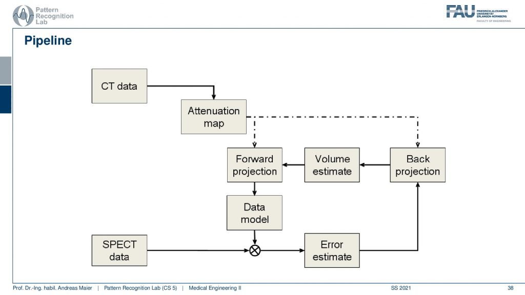
Now the actual reconstruction then often looks like this. So you acquire a CT data set and the CT data set is relevant because it tells us how much the body actually attenuates. So it will tell us the topology of the body and where we would lose more γ quanta when they pass through this part of the body. So we need a CT scan and this gives us an attenuation correction map. Then this is a mapping here because typically we have a different kind of acceleration voltage in the CT scan than the γ quantum that we have in the PET or SPECT scan. So they have to be calibrated to be in the same energy range and then we get an attenuation map that tells us where we are more likely to lose photons. Then we have the SPECT data and from this, we can start an initialization. So we start then with a first initial guess, forward project this volume, and get an estimate of the projection. Compare this to the actual projection data. Then we estimate the error. This error is going to be backpropagated. So we update the activity in the volume. This gives us a new volume estimate which we forward project and then we get essentially this loop and we iterate until convergence until the only small changes or a fixed number of iterations is reached and this gives us then the final image reconstruction. Let’s have a look at different reconstruction results.

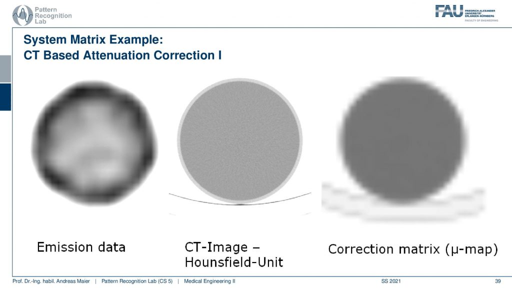
What you have to keep in mind is that you have some emission data. Then you have the CT scan. You see the resolution of the CT scan here is much finer. So you see that it has a very very fine resolution. This is used to produce this kind of correction map or correction matrix and this is also called μ-map. You see that we have to reduce the resolution of course and we have to adjust the attenuation coefficients because they are different in different energy ranges. But this can be done with a linear estimate. So it’s not that difficult if you already have the CT scan. 

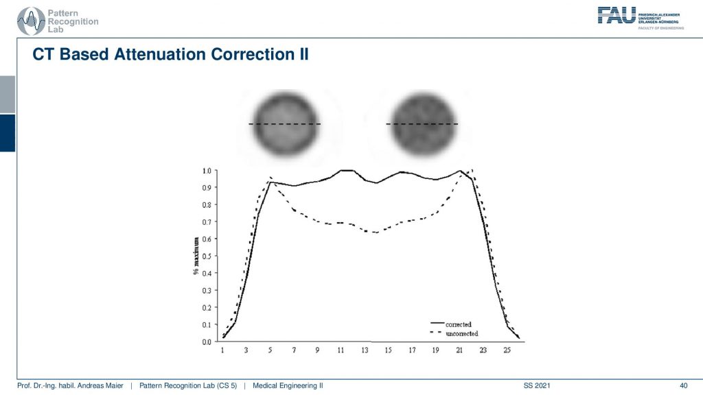
Now if you do that then you can do two different kinds of reconstructions and here we are comparing a reconstruction without attenuation correction and with attenuation correction. You see very clearly if you don’t correct for the attenuation, you get this kind of cupping artifact. If you do perform attenuation correction using a mu map you get a very homogeneous intensity and obviously, this is a cylinder of constant activity. So we would like to reconstruct a flat plateau-like this one and what you see here is the intensities along this line here. So this is what the attenuation correction does. Then we can also look at an advanced principle. 

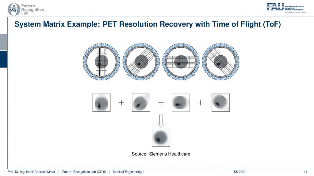
This is called the Time of Flight principle and PET and there are very very fast coincident detectors. They’re not just able to detect which events actually happen at the same time, but they’re even better. They can detect the time shift between the two events. This allows us to locate the wind not just to a certain ray but also to a certain depth. So from a single time of flight measurement I don’t just get the actual activity, but I also get a depth estimate. So from a single projection that I synthesize from several elements in a certain direction, I can reconstruct the back projection that is already resolved with respect to depth. Then I can do that for multiple kinds of directions and in contrast to what we would see in a classical back-projection where everything is just smeared across this direction. We can get a very much improved resolution characteristic for PET images. So this Time of Flight imaging is a very nice tool to detect where actually on the ray connecting the two detector elements the event has happened and I can supply it with an additional depth direction. So that’s pretty cool! So we can get much sharper images using Time-of-Flight technology. 

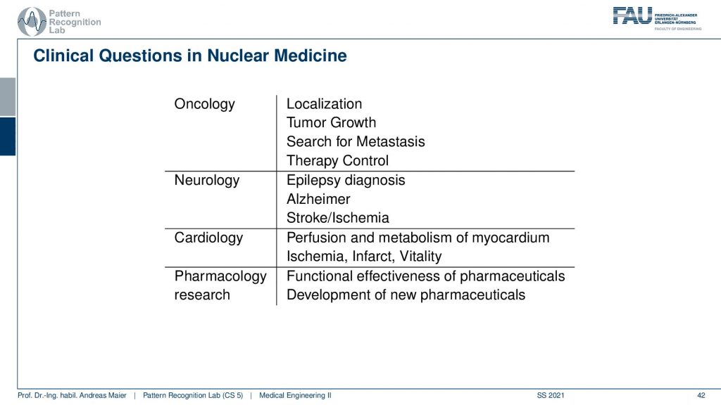
Now we want to use that for clinical questions and what is typically being investigated is in oncology you localize tumors you can also localize metastases. You can quantify tumor growth. You can search for metastases and you can use them for therapy control. In neurology, you can diagnose epilepsy Alzheimer and stroke. In cardiology, you can check the perfusion and metabolism of the heart and detect ischemic region infrareds and the vitality of the heart in general. Also in pharmacology research, you can essentially assess the functional parameters of pharmaceuticals and how they change the metabolism. So this is also a very relevant kind of research where PET and SPECT imaging is being used. 

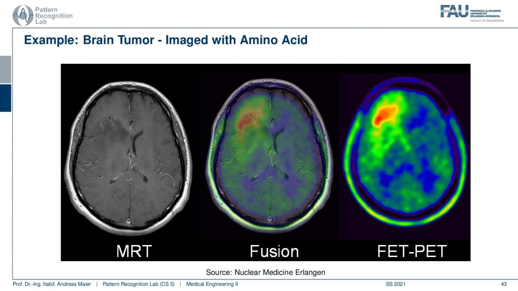
Now here I have a couple of interesting overlays. So this is an MRI image and here you see a kind of PET image and this PET image now shows essentially different information and I can fuse them. So I can bring them into the same coordinate system. Then I can see with a structural background that actually this kind of activity is associated with this brain area and here I know the brain area is very low in this image. It’s very hard to differentiate the brain areas. So the joint use of two modalities brings us much better localization properties with the nuclear imaging scans.

So most of the scanners that I use today are actually hybrids.

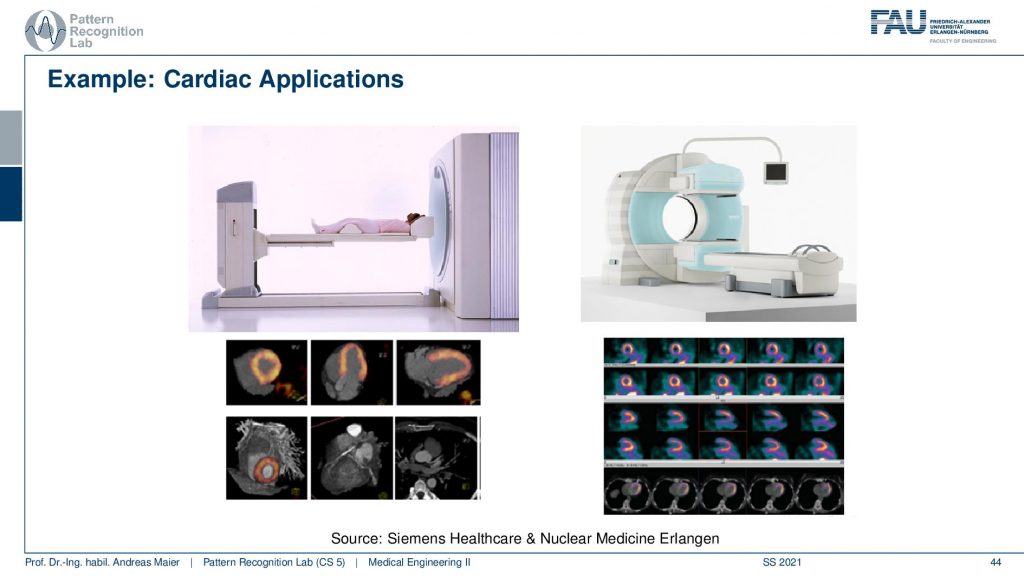
So there’s either the PET CT or the PET MR. So you can associate the scanners with different other modalities in order to get the additional localization information and this is the workload of the scanners thereof the hybrid systems. So are some cardiac applications and you can see here that the myocardium can be imaged with scanners and these are different scanners from siemens healthineer. You can also see the kind of distribution of the tracer in the heart muscle and then if you see that there are areas where the tracer is actually going very well. Then this is typically an infrared area where there is not enough blood supply and therefore also the heart is malfunctioning. So that’s a very popular technique to assess the heart. 

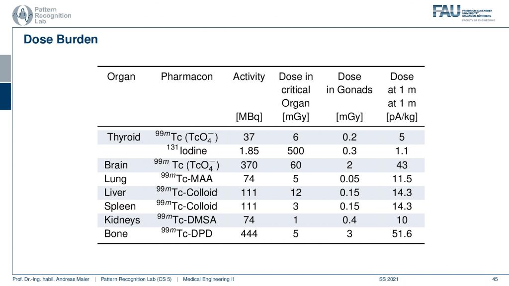
Obviously, there is also some dose burden associated with a different kind of diagnosis. Here you see for example in the thyroid you have a certain activity in MBq. Then you can also determine a critical organ dose and for example the associated activity in other organs. Obviously, if you move closer towards that specific other organs then the dose version also increases. So what’s very classical if you do such a scan and in particular also if you plan therapy, then you segment the organs and you try to predict how much dose will go into other organs. Then you can use that to adjust the amount of therapeutics that are being used in order to fight for example cancer or so on.

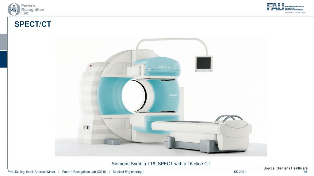
Let’s continue and talk a little bit about hybrid imaging. So I already said that most of these systems are hybrids today. In SPECT you very often have combinations with CT. So you see this is the SPECT camera and this is the CT system. So this is a CT gentry. This donut and you can image CT and SPECT at the same time. 

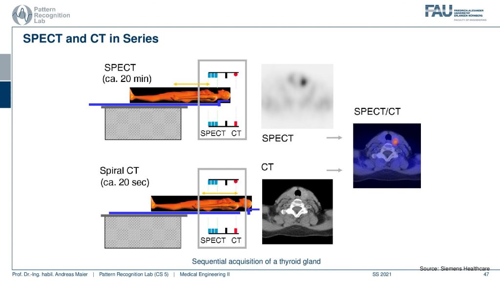
So the way of how this is being done is you put the patient on the table. Then you do a 20-minute SPECT scan and then you can do a helical spiral CT by moving the patient here. So you see this is the CT gantry and this is the SPECT gantry and then you don’t have to move the patient remains in the same position. Therefore then you have two scans that you can overlay very well. I mean this is very important if you image the abdomen. Because if you have the patient stand up and sit down again and all the organs shift around and this would make the retrospective registration of the two scans very difficult. So you want to have the patient lying on the same bed when you do those two scans. Obviously, there’s also breathing on top. So you still may want to register the motion and compensate the motion between the scans but this can actually be done on top of these hybrid systems. 

Another alternative is PET/CT.

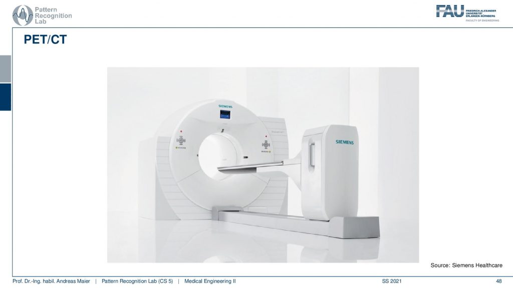
So here you have a PET ring and a ct gantry that are just in the same kind of donut and then there is also the PET/MR.

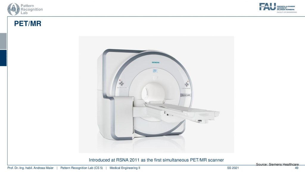
This is now a very long system. So you have a PET ring and an entire MRI machine here and this system can simultaneously acquire MRI and PET. This is also very cool because the MRI scans can also take rather long. But you can image long protocols and also very frequently update motion parameters and things like that and this allows very accurate motion compensation in these systems. So it’s a very cool technique! 

But one thing that you don’t get from MRI is the μ-maps. So, you don’t get the attenuation correction and this was a huge problem actually when they were designing these systems. But it turns out that you can use ultra-short echo sequences. So you actually have a set of four sequences the Dixon water, Dixon fat, and then different ultra-short sequences and with that, you train a machine learning algorithm and you train it in a way that it predicts the CT image. So already when the first PET MR scanners were introduced they were shipped with machine learning that would predict the attenuation maps from different MRI sequences. So that’s pretty cool and we’ve seen that the world of medical imaging and machine learning are closely related together. Actually, the algorithm that has been used in the PET MR scanner has been manufactured first. This kind of system had an algorithm that was co-developed at our lab as well. So that’s a pretty cool development and we see that these algorithms are crucial if you want to build a sophisticated system that can do attenuation and correction. It’s also pretty nice that actually, the absorption that we have in CT is very different from the MRI signal. Still, we can use the similarities in anatomy and the location of the image patches to predict reasonable μ-maps. So that’s pretty cool. So we can predict something that we never physically measured just by using the prior knowledge about anatomy and how patients typically look like to get a coarse estimate that is good enough to get an attenuation correction that is very very close to using the original CT values. So that’s also a very nice result and this essentially enabled using MR scanners in hybrid PET installations. 

So this already brings us to the end of this video. So you’ve seen the principles of nuclear imaging and how we can use tracers. They get essentially connected to certain molecules that are important for metabolism. Then I can watch over time where the tracer is going and analyze the function of the metabolism of the body and with that, we are then able to analyze specific diseases. We’ve seen that we can not only use that for cancer, but also for brain diseases for Alzheimer’s and also for diseases in the heart. So this is a very important technology that allows us to assess how well the function of the body actually works. And we can do that entirely non-invasively. Well, there is a certain dose burden but if you look at the types of disease that we have they typically appear in elderly persons and therefore there is only a little tracer being used. Also if you already suffer from cancer, the risk of developing cancer in 10 or 15 years from the treatment may not be as acute as actual cancer that is currently growing in your body. So these kinds of technologies help us to improve the care of the patient the treatment and we’ve seen that we can use them also for diagnosing severe disease and for planning respective treatment. So I hope you enjoyed this video and this small excursion into functional imaging. This already ends everything that we talk about functional imaging here and instead, we want to look into the next modality in the next video and this is going to be ultrasound. So thank you very much for watching and looking forward to seeing you in the next video. Bye-bye!!

If you liked this post, you can find more essays here, more educational material on Machine Learning here, or have a look at our Deep Learning Lecture. I would also appreciate a follow on YouTube, Twitter, Facebook, or LinkedIn in case you want to be informed about more essays, videos, and research in the future. This article is released under the Creative Commons 4.0 Attribution License and can be reprinted and modified if referenced. If you are interested in generating transcripts from video lectures try AutoBlog

References   

• Maier, A., Steidl, S., Christlein, V., Hornegger, J. Medical Imaging Systems – An Introductory Guide, Springer, Cham, 2018, ISBN 978-3-319-96520-8, Open Access at Springer Link

Video References

1. Doktor Klioze – PET Imaging https://youtu.be/k2jnSmpHqzg
2. Automatic Collimator Changer https://youtu.be/E_zpIOzq9xM
3. Medical image Registration https://youtu.be/ZOlRVpOj9Vg

Category: Lecture Notes in Medical Engineering