Ultrasound

These are the lecture notes for FAU’s YouTube Lecture “Medical Engineering“. This is a full transcript of the lecture video & matching slides. We hope, you enjoy this as much as the videos. Of course, this transcript was created with deep learning techniques largely automatically and only minor manual modifications were performed. Try it yourself! If you spot mistakes, please let us know!

Welcome back to Medical Engineering. So today we want to talk about ultrasound. This is a key imaging technology and it’s very broadly used. It’s also a very safe imaging modality and it can be used to diagnose many many different diseases. We will see that it is also very versatile and we can use it also in acute scenarios because by now the imaging modality has already been transferred into rather small systems and some of them are portable. So looking forward to exploring ultrasound with you guys. 

So let’s start talking about the ultrasound applications and we actually want to figure out where ultrasound has been being used before it actually emerged to become a medical imaging technology. So this then leads us to ultrasound and medicine and later we want to use this knowledge about the physics of the waves to understand how the actual ultrasound image formation is done. This then brings us to understand the different purposes and the different applications of ultrasound in medical. Finally, we want to have a short consideration of the safety of ultrasound in imaging.

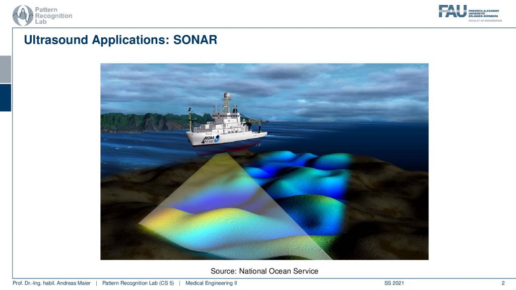
Well, where are ultrasound being used and one of the earliest applications actually sonar and here you see an application where we can try to analyze the height of the ground in the sea. One of the earliest applications of ultrasound was actually in the war to detect enemy submarines. So this is one of the technologies where it became very very relevant in order to figure out where your enemy is. Of course, ultrasound is also used in other applications. 

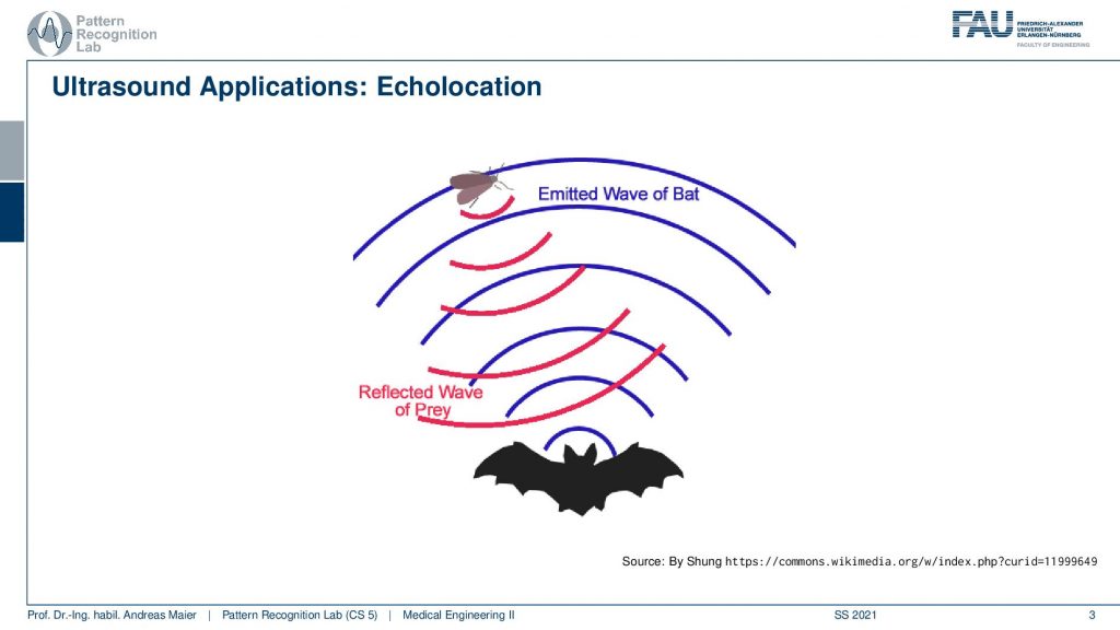
You may of course know that bats use ultrasound in order to figure out where their prey is and they use echolocation. They send out this ultrasound wave and then they have these large ears and with the ears, they can hear where the reflection is actually coming from and this enables them to detect their prey also in conditions where there is very little light. So they can fly around and then hunt insects also in very dim light conditions and therefore also ultrasound is a very commonly used technique in the animal kingdom. 

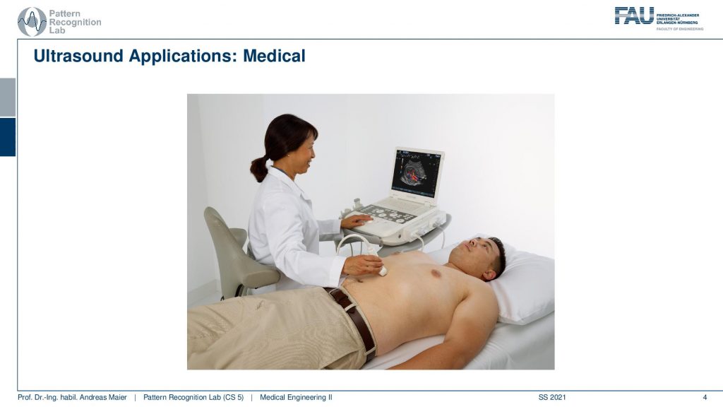
Now we want to use ultrasound for medical applications. Here you see a typical scenario that you may have undergone or have not undergone and here you see that you have this ultrasound probe and with the ultrasound probe you locate the region of interest inside the body. Then you use it in order to visualize essentially instantaneously the image on the screen and then you can make your diagnosis. 

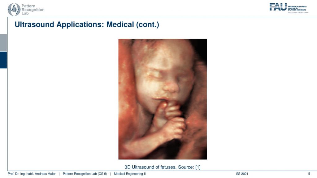
There’s also 3d ultrasound and here you see an example that is used in maternity care. So you can here see the fetus before the birth and you can essentially use this technology to visualize the phase of the growing child during pregnancy. So you can already meet your unborn child. So this is also for parents or soon-to-be parents a very important technology that you can take care of the growing child and that you are aware of any problems that may emerge during pregnancy. 

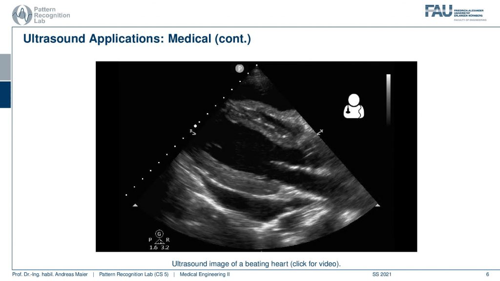
So what you also do with ultrasound is that you also image internal organs and here you see an application of the beating heart. There we already see a couple of the challenges of ultrasound. So you have to look very closely here in order to see anything. You have to know where you’re placing the ultrasound probe. So if you don’t, then it will be very difficult to figure out the anatomy. What you can see here is that first of all there’s a caption saying that it’s the beating heart. It always helps me and then you can also see that there are essentially the heart muscles here and you see that there are areas where the blood is flowing. So you see some of the heart chambers. But it helps to have some anatomical knowledge such that you know how the heart is positioned inside the body that you can figure out what cross-section of the heart you’re currently seeing. So all of these are cross-sectional images and what ultrasound is also very famous for is all of the speckle noise that is emerging here. So it’s rather difficult to work with the modality and you have to have very good anatomical knowledge if you use it and want to see the right thing.

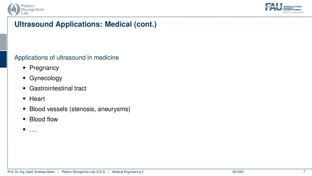
So this is a classical ultrasound image and it’s used in all places of medicine in pregnancy and gynecology in the gastrointestinal tract, in the heart and blood vessels, and for analyzing the blood flow.

So there are plenty of applications with ultrasound. Now let’s have a look at ultrasound in medicine. 

Ultrasound in medicine has been used essentially as a development from the first ideas in the use for detecting submarines. Then we found that it can also be used to explore not just finding enemy submarines but you can also use it to find the inside of the body. 

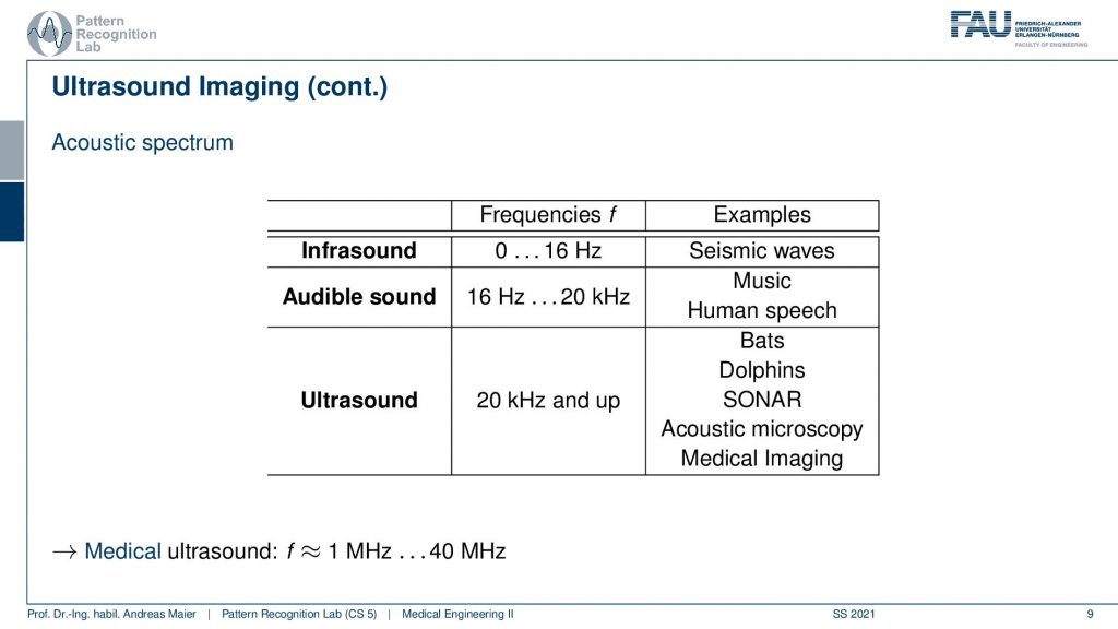
If you take a look at different acoustic waves you can see that there is infrasound and infrasound is somewhere between 0 and 16 Hz. So this is a very low frequency and for example, seismic waves are in this kind of frequency range. So you rather feel that shaking then actually you can hear that. So there’s a certain limit to the frequencies that you can hear and then starting from 16 kHz you start perceiving this. So this is audible sound and we already discussed that it’s approximately from 16 Hz to up to 20 kHz and this also gives then rise to determine the sampling frequencies for music on the compact disc. So this is music human speech that is in this frequency range. Everything beyond 20 kHz is ultrasound and this is where bats dolphins also orcas communicate in this frequency range. This is also where we place sonar acoustic microscopy in medical imaging. For medical ultrasound, we are typically in the range between 1 to 40 MHz. So these are classical frequency ranges for the ultrasound. 

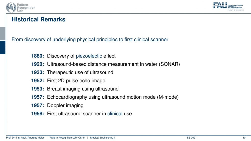
Now let’s talk a bit about the history from the discovery of ultrasound to the actual manufacturing of medical-grade scanners. So first we had the discovery of the piezoelectric effect which was very relevant in order to produce these kinds of waves very quickly. So we’ll see that in a bit why it’s relevant. Then the ultrasound-based distance measurements in water sonar. Then we had the first therapeutic use of ultrasound. So you actually use it to alter something inside the body. So you need strong pressure waves. Then you can for example break down certain stones inside the body. So that would be a therapeutic use. You can also create heat by the way and this is also something where highly focused ultrasound is also a therapeutic kind of intervention. There are for example experiments that you can target certain tumors with focused ultrasound techniques. Next thing is that the first 2D pulse-echo image was generated in 1952. Followed by that the first breast images with ultrasound and then echocardiography has been done with ultrasound and this gives rise to the motion mode. We will discuss that also in a couple of slides. Doppler imaging takes effectively the acoustic Doppler effect and allows us to measure essentially flow and finally here in 1958 the first ultrasound scanner is in clinical use. So all of these steps had to be taken in order to develop a medical-grade scanner. 

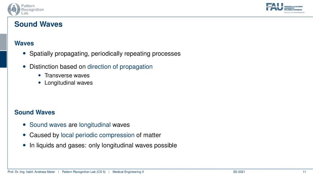
Let’s have a look at the physics of sound waves. You already have seen it very frequently here in this lecture with respect to light or also with respect to x-rays and so on and there we have essentially spatially propagating periodically repeating processes. There is a difference in the acoustic waves because they’re the direction of propagation is different. They’re transverse waves and there are longitudinal waves and the sound waves are longitudinal waves. So the direction in which they are propagating and the direction of the pressure change is the same. The reason why they emerge is that there is a local periodic compression of matter and this causes a wave to be spread through the medium and in liquids and glasses only longitudinal waves are possible. 

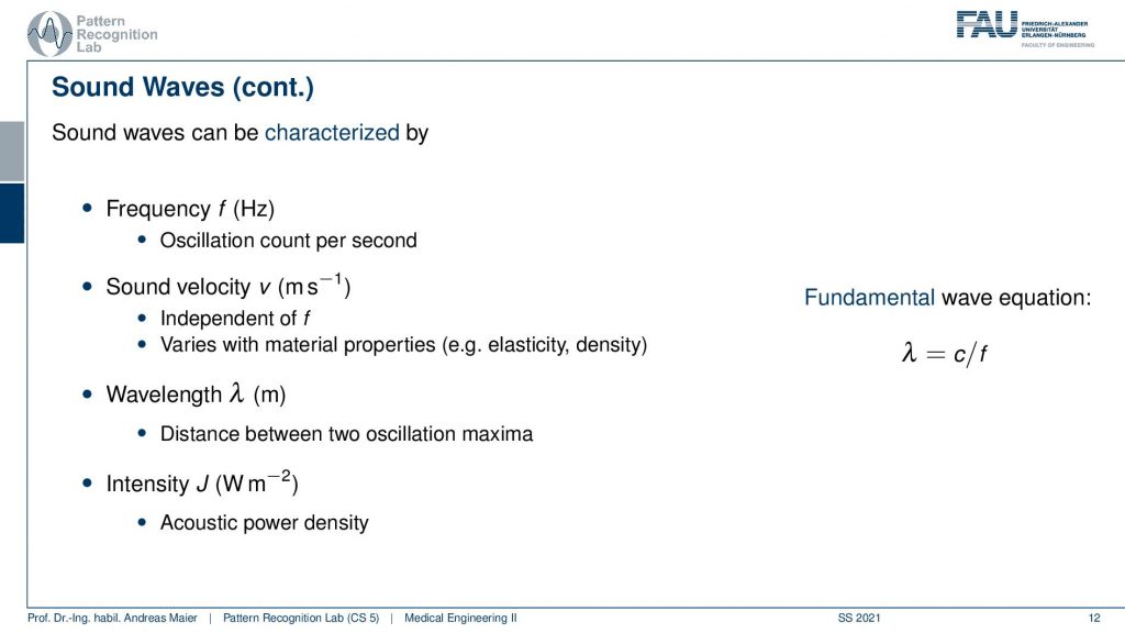
So typically we can characterize those waves with a frequency that is essentially a number of oscillations per second. We have the sound velocity and this is independent of the frequency and tells us how fast the sound waves propagate into the medium and it varies with the material. So, in air, you have a different speed of sound than in water. In water It’s the denser speed of sound propagation is much faster. This then leads us to the concept of the wavelength which is essentially the length of one wave and this is the distance between two oscillation maxima. What’s also very relevant is the intensity and here this is measured in Wm^-2 and this is the acoustic power density. Also, the fundamental wave equation is present here. So the wavelength can be determined from the speed of sound in the respective kind of medium divided by the frequency. 

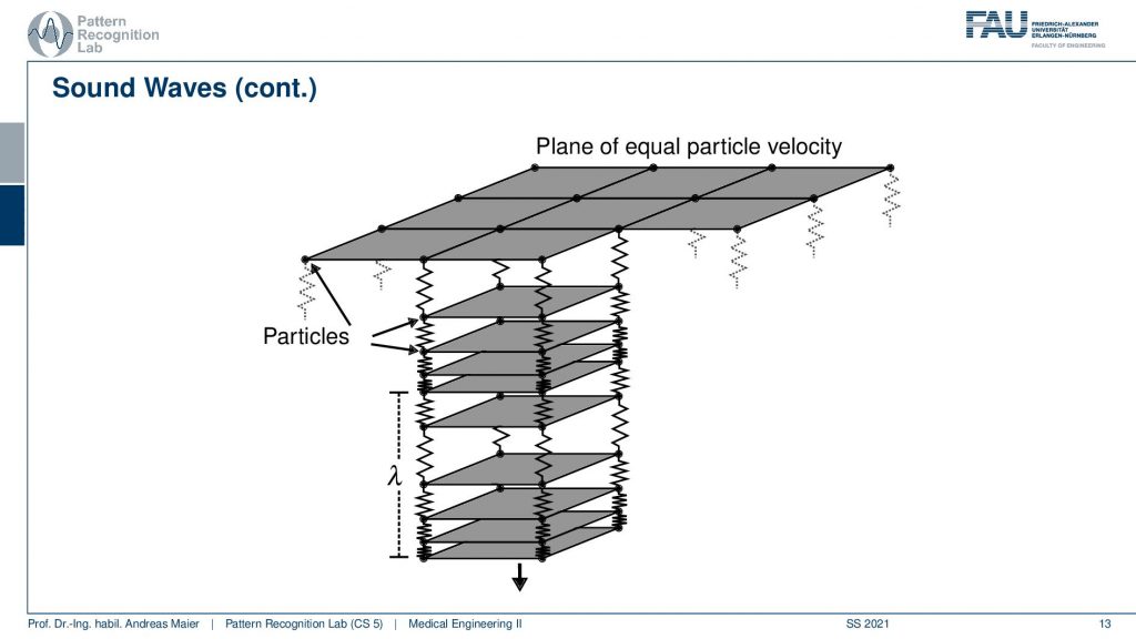
Let’s have a look at a conceptual study here. So this is essentially a medium and we show this by a set of planes. In order to think about how this wave propagates, we can think about the particles in our medium being connected with tiny springs. So these are springs and they connect the different particles. Now if I start pushing here you can see that the distance between the particles reduces and expand and I have to have some kind of oscillating pressure here. Then this will cause this to propagate inside of the medium and the distance between two maxima here and here is exactly our wavelength lambda. So this is a kind of busy plot. 

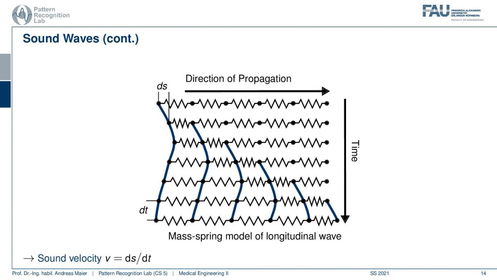
We can simplify it a little bit if we only look into the propagation direction and into the time direction. So now we can understand how the wave behaves over time. So we start essentially weakening here. So we push and expand and this then causes our wave to propagate over time. So it moves in the direction of propagation with additional time. So you can see how it moves along the time axis. So this is how the wave propagates through our medium. Then we can determine the sound velocity which is the step length over the time segment and this can essentially characterize how fast the wave is propagating. 

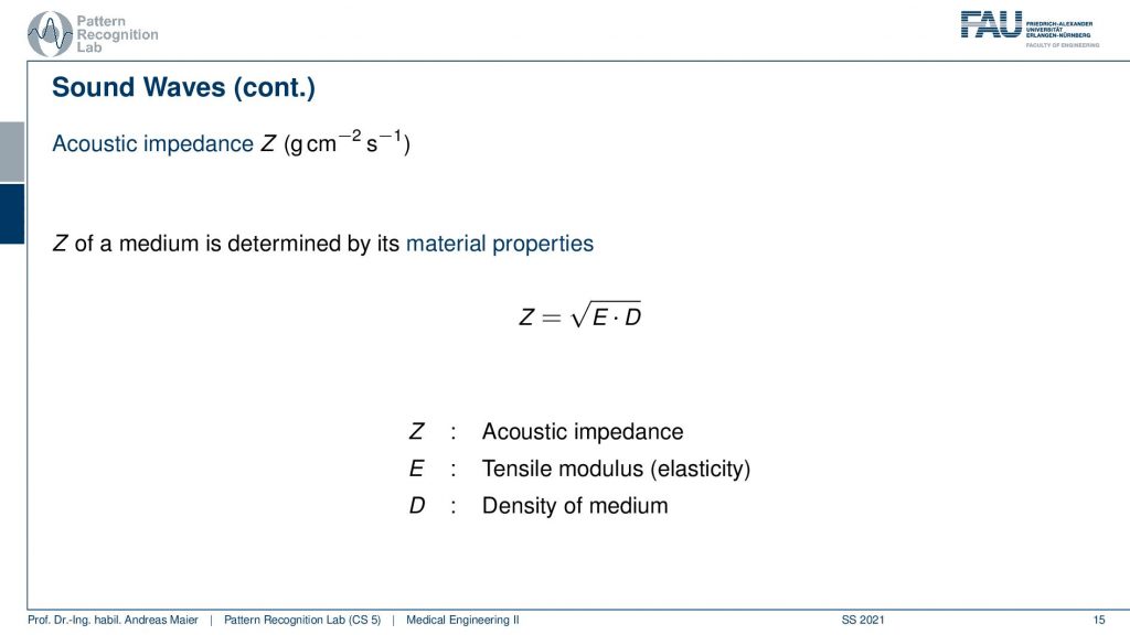
So we now have to talk about a couple of additional concepts that are very relevant for this propagation effect and important is the so-called acoustic impedance. This value z here is measured in this physical quantity and the acoustic impedance of a medium is determined by its material properties and there are two of them that are relevant. This is the tensile modulus the elasticity and the density of the medium that tells us what the actual z here is. The acoustic impedance is very important to understand the actual propagation in that medium. 

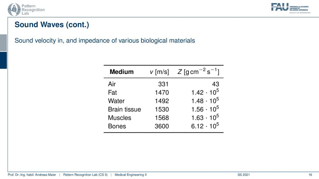
Let’s have a look at different kinds of acoustic impedances here. So this is z and we see in the air we have an acoustic impedance of 43. A sound velocity of 331 meters per second and you see that in the soft tissues here. So this is fat, water, brain tissue, muscles, and bones. You see that in the watery tissues these guys here of course a little bit denser but we have a much faster speed of sound here. Also in the very dense bones, we have an even faster speed of sound. This then also takes effect in the acoustic impedance. You can see that in the watery tissues here, they are approximately in the same ballpark with 10^5, and then you see the acoustic impedance here in the bones. It’s much higher. So this is approximately four times higher than the watery tissues. There’s a huge mismatch with the one in air and this is orders of magnitude different. You have to keep this in mind and if you want to understand why certain propagation effects happen. So keep that in mind air is very different than the watery tissues and bone is very different than all the other materials that we mentioned so far. 

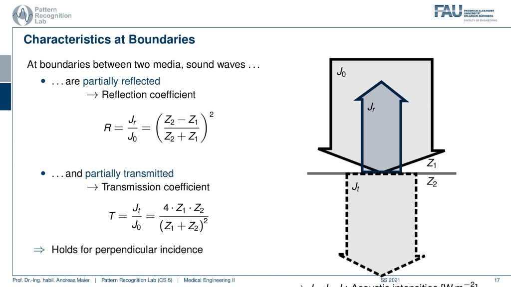
This brings us to the effects that happen at the boundaries of different tissues. At the boundaries of different tissues, there are a couple of things that can happen. Partially the wave will be reflected and partially the wave will be transmitted. The reflection and the transmission coefficients are dependent on the acoustic impedance. So you see this is all constructed on the acoustic impedance of our material 1 and material. 2. so the difference in the acoustic impedance essentially causes either reflection or, transmission. What you can see here is that you add the two and you subtract the two divide and take it to the power of two. So if you look carefully here this is the intensity that is going to be reflected and this is the intensity that actually reaches the boundary. So if I have a large R and this R is close to 1 then almost everything is being reflected. Now if you have two different acoustic impedances and the difference is very large. So let’s say this is 43 and this is 10⁵ and then you see that the difference here and the addition of the two will be very close. So this is going to be very close to 1 and if I take 1 to the power of 2 it will stay at 1 meaning if I have a large difference between the two I will almost only observe reflection. On the other hand,  if I want to compute the transmission coefficient I have to multiply the two and if there is a large difference between the two and I divide by the sum of the two, we will have something that will be very low. So there’s almost nothing transmitted. If I have values that are approximately in the same ballpark, then obviously I get really transmission and I don’t get so much reflection. Now you remember that we had a huge difference between air and watery tissues. So if you have any intersections between air and watery tissues or, an intersection between bones and watery tissues almost for sure you will have a complete reflection. So the wave will not penetrate but it will get reflected. So this is then also the reason why you use this kind of gel on the transducer on the ultrasound probe when you want to get a signal because you have to be sure that there is no air between the transducer and the body. If you don’t use this gel then you might have air in between and the air then gives a total reflection and you don’t get any signal. Also, you have to move your ultrasound probe in a way that you image through the bones. Well not through the bones not transmitting through the bones but in between the gaps between the bones. So if you image through the torso, then you want to find gaps in between the ribs in order to get good images. If you try to image through the bone then you will almost for sure get a total reflection. So this is also why ultrasound is very seldomly used in the head. So you’re only using ultrasound in areas here in the neck. So you can have a look at the carotid arteries and stuff like that but as soon as you want to look into the skull ultrasound is not the modality of choice. So keep that in mind. This is all related to acoustic impedance. 

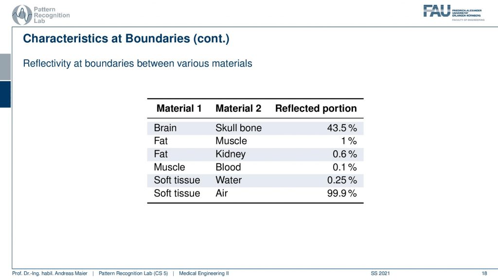
Okay so now that we understood this, then we can also have a look at the different reflection portions. We can already see it here with brain and skull bone 43 soft tissue and air 99.9 of reflection. So really a high value and you can compute all of these numbers from the previous table. So we can go ahead and check whether the numbers are right. 

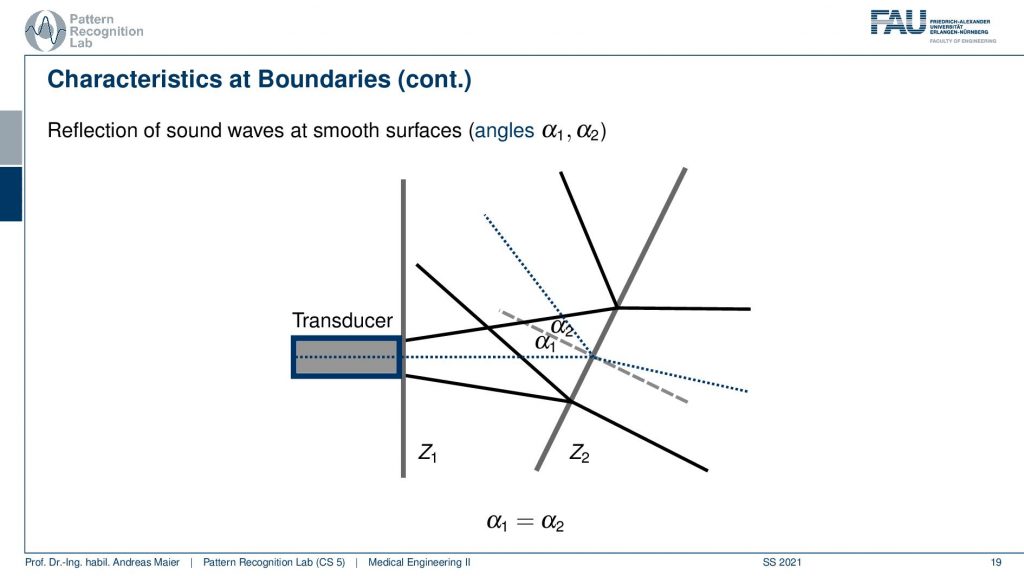
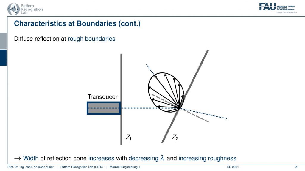
Now we understood the reflection then there is another thing happening and this is the reflection of sound waves at smooth surfaces. So what happens is if I have a wave propagating and then there is a smooth surface? What would happen is it would get reflected in a different direction. Now in the body, this doesn’t happen because what’s happening in the body is you never have a perfectly straight line here but it’s always a kind of not straight surface that’s happening. 

What’s now happening here is that you get some reflection but it also gets some reflection back. So this can also help us with getting the signal back and measuring it. Okay so now we understood why there are reflections and why the sound waves propagate. 

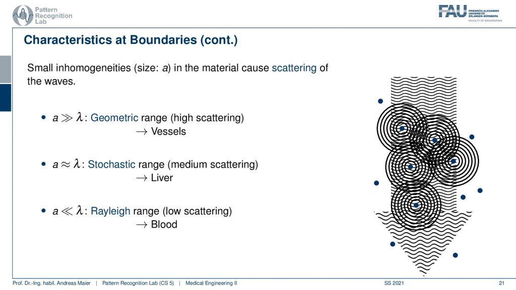
Another effect that you want to keep in mind is the scattering of the waves. If you have essentially material or, structures in the body that is approximately in the size of the wavelength, then you get a stochastic medium scattering. So you get scattering all over the place. If you have the wavelength much lower than the size of the inhomogeneity, then you get geometric scattering and this happens for example at vessels. Then there’s also Rayleigh range. So there the wavelength is much larger than the scatterer and this happens for example at blood and you get some very low scattering. With these scatter effects in mind, we can now kind of summarize this.

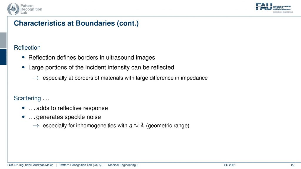
There is a reflection that’s happening and there’s scattering that’s happening and all of this then adds up to the different effects that we see in the image. In particular, we will have to use reflection in order to figure out what’s going on in the body. So this is something that we will see and this especially happens at borders and especially with large differences in impedance. It’s also the reason why we need to use the gel and the scattering is one of the noise sources that you see in the image and scattering is actually a very crucial factor in ultrasound. 

Another effect that we have to keep in mind is attenuation.

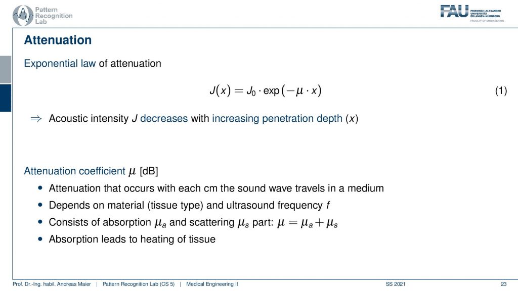
Attenuation is also happening. So here our J also decreases with the depth that we penetrate and there is μ that is this kind of absorption coefficient. This attenuation coefficient is actually dependent on the ultrasound frequency and on the tissue type. We’ll see that is an important thing because the attenuation is different with the frequency range and this essentially determines how far we can actually penetrate different tissues because of the different attenuation effects. You see that there is also exponential decay dependent on this attenuation factor. So what happens if stuff is being absorbed. Well, it leads to heating of the tissue. So this is also why there is some heating but typically in the normal imaging that we’re doing, there’s almost no heating. So you would have to do a very long ultrasound that you do heating. 

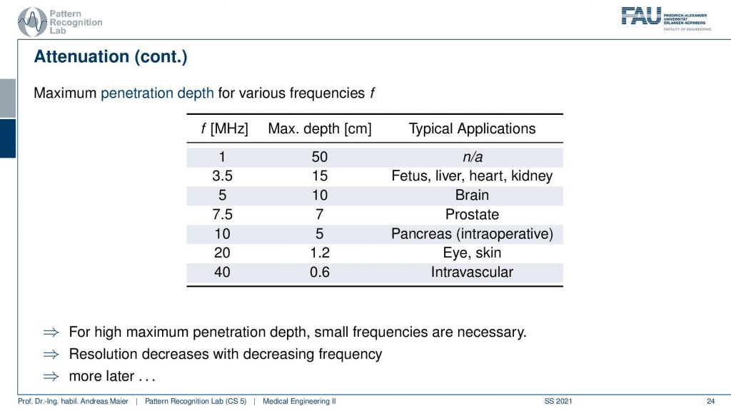
We see that the frequency is very important in order to determine the maximum depth. So with 1 MHz, I can get up to 50 centimeters of depth with 40 MHz, I can only penetrate 6 millimeters. So here we have very strong attenuation which means we can only penetrate very little at this high frequency at the low frequencies, we can penetrate much deeper. So you see then this has different applications and for intravascular for eye and skin we use the high frequencies and for fetus liver brain we kind of take the lower frequencies. So for maximum penetration depth, you take a small frequency and for high frequencies, you only have a low penetration depth. We will talk about this in a couple of slides again.

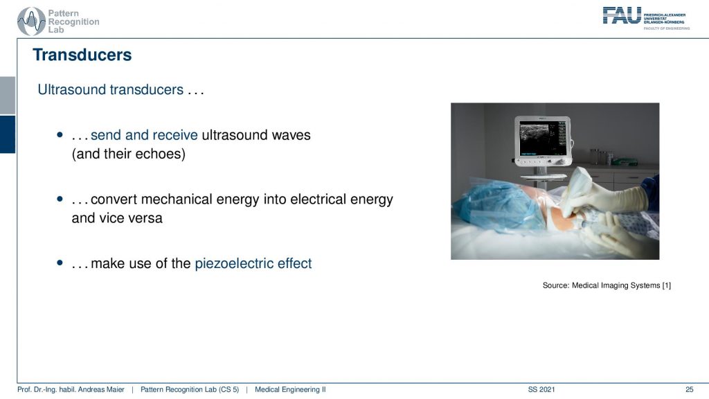
So now we have these ultrasound transducers and we somehow have to send and receive the ultrasound waves. We have to convert the mechanical energy into electrical energy and vice versa and this uses the piezoelectric effect. Now, what’s the piezoelectric effect?

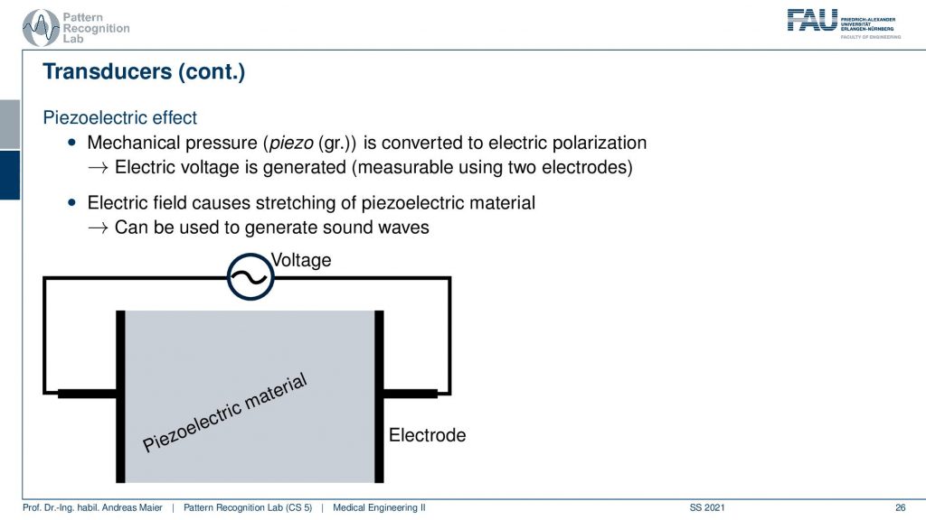
 That’s actually such a crystal here. This is a piezo crystal and if I apply a voltage it will expand and this happens almost instantaneously. So this is very nice. Then I have this expansion and then I turn off the voltage and it goes back. So I turn on and off the voltage all the time and I can create these pressure waves. So I can essentially convert an electric field into a kind of pressure wave and I can convert a pressure wave into an electric field with this kind of effect. 

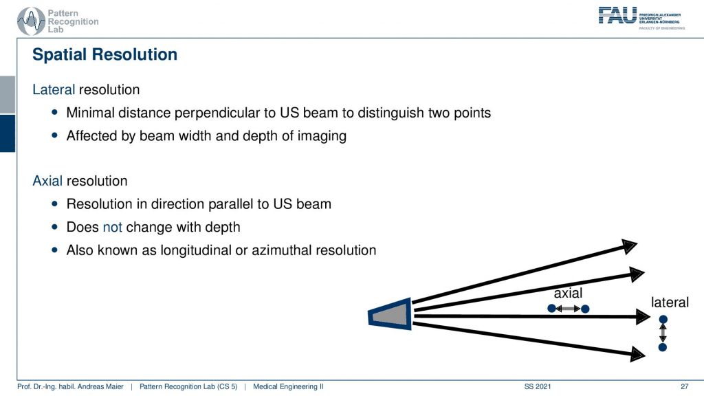
This is nice. Then of course we can do different spatial resolutions. And there’s of course the lateral resolution and the axial resolution. Now the lateral resolution is dependent on the design of the transducer. So how many transducer elements do we have and how many waves can I send out in different directions. The axial resolution does not depend on the actual design of the transducer but it is dependent on the frequency that we are actually using. So this is the resolution in the direction parallel to the ultrasound beam. This is the axial kind of resolution. It doesn’t change with depth and it is also known as the longitudinal or asymmetrical direction. 

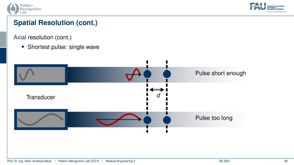
Now if we want to understand how we can resolve the axial effects, we have to understand how the waves are propagating through our tissues. If I have a short wavelength which means a high frequency, I have shorter waves and they essentially go into our tissues. Then there is some interaction here and another element here and there are separate by the distance d. Now I have the case of a long wavelength and a short wavelength. Now I send them into the tissues and what now happens is that they get reflected. In the above case, I can see that two waves are coming back one reflected from here and one reflected from here in the lower case, you can see that the distance is shorter than the wavelength and I can’t differentiate anymore. It’s the same way for a different wave because there is no distance in between. So higher I pick the frequency the better the resolution in the axial direction gets. 

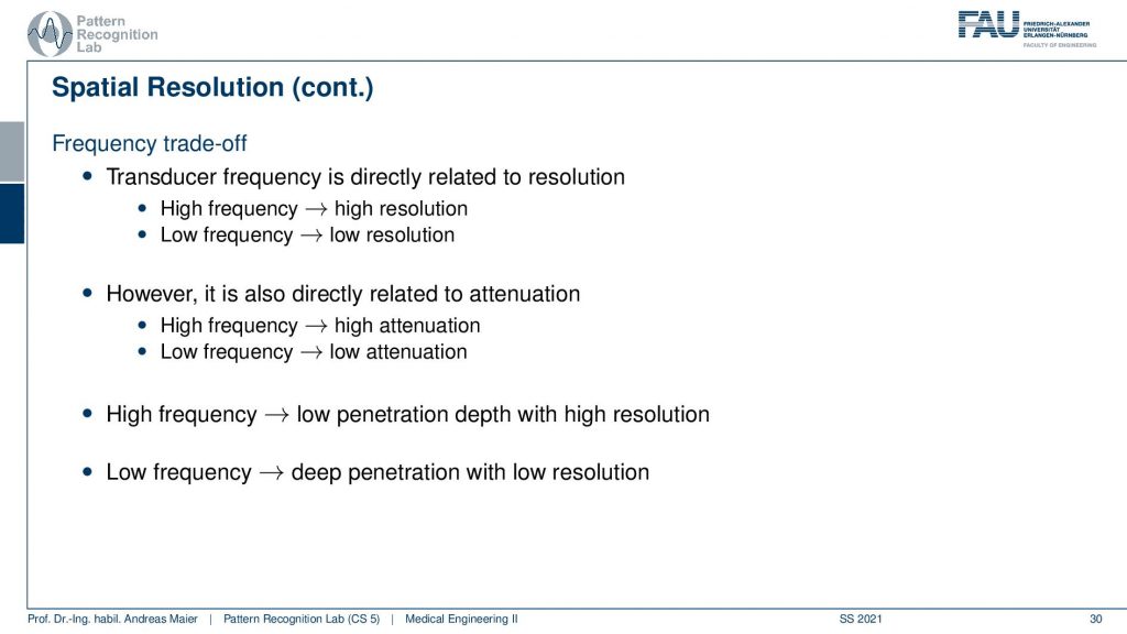
This then leads to a frequency trade-off between high-frequency high-resolution low-frequency low resolution. But it also depends on the attenuation. So if I have a high frequency I have high attenuation and if I have a low frequency I have lower attenuation. This means high frequency leads to low penetration with a high resolution and low frequency leads to deep penetration with low resolution. So this is the trade-off of the frequencies and then you can also understand why we have these characteristic frequencies for the different organs because they also have a characteristic size. This then tells us what kind of frequencies we can use and actually how deep we can penetrate the tissue. 

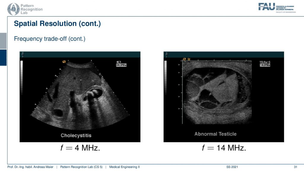
Let’s have a look at some examples here. Now you see here a 4 MHz image and this is a Choleocystitis. And here you see a 40 MHz kind of image and this is imaging an abnormal Testicle. So you see that the size here is very different and this is dependent on the frequency. So let’s talk a bit about the imaging modes. 

So we now understood how things are reflected. We understood about the acoustic impedance and why we sometimes have total reflectance and why we need shorter wavelengths in order to get higher resolution. Now let’s see how we can image with these different setups.

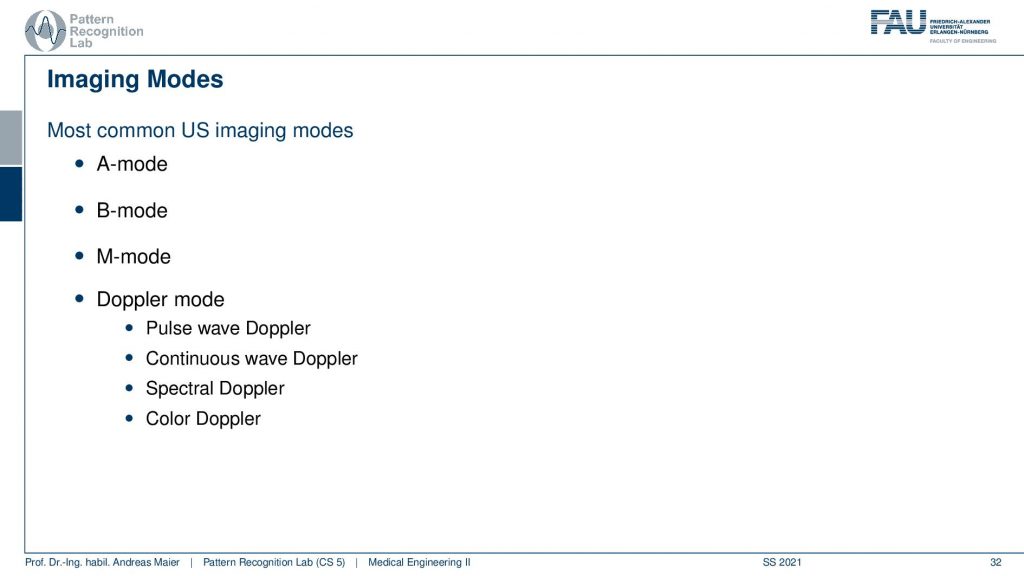
There is essentially a couple of modes. So there’s the A mode the amplitude mode the B mode. This is probably what you know as an ultrasound image. There’s the motion mode. This is time-resolved. Then there are the Doppler modes that essentially tell us that we have an acoustic Doppler effect and it allows us to measure propagation speeds and flows for example of blood. So there’s spectral Doppler, color Doppler, continuous-wave Doppler, and so on. But we won’t look into all of these details. 

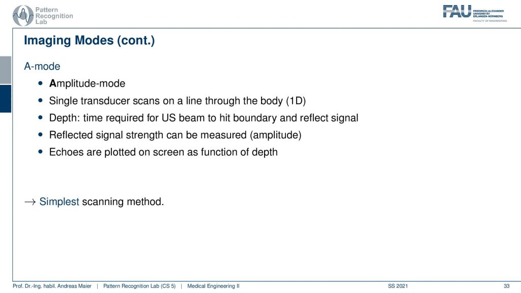
Now the amplitude mode is essentially an A-scan and this is only a 1D signal. So there we only have one transducer element and we scan essentially one dev profile. This is the amplitude mode. This is the simplest scanning method and then you plot the echoes on the screen as a function of that. So what you get is then the depth here and then you have some echoes. This is just a single-line profile. Now that’s not so interesting but of course, we can arrange multiple of those eight scans, and now this is where the different transducers come in. 

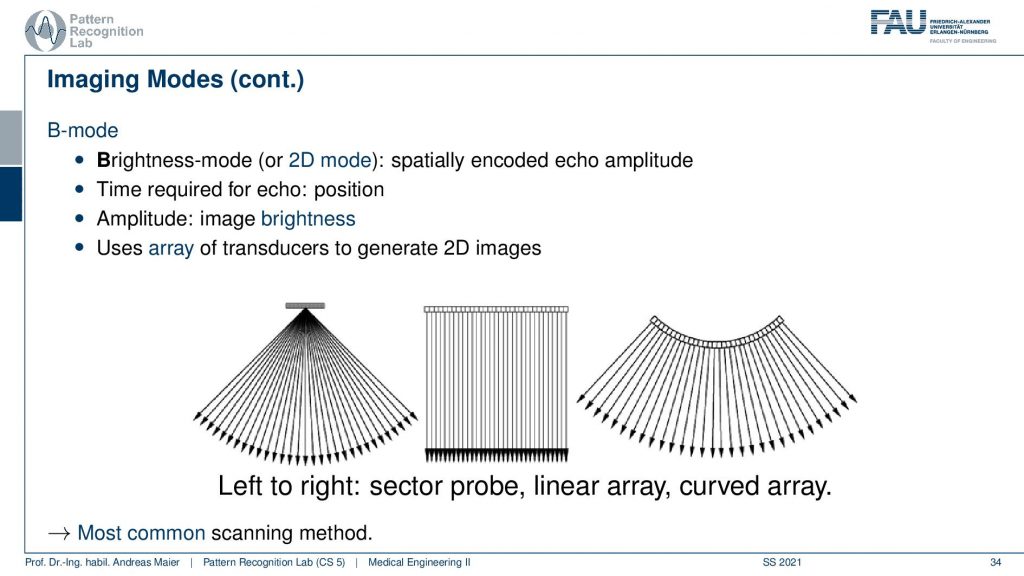
So you can then align the A scans in different geometries. So you can get this fan-like structure, you can get a parallel beam structure or, you can also have a kind of open fan structure like this one and this is probably what you see in most of the transducer heads. So this is the most common scanning method and this yields 2D images by constructing this array of transducers. Here we have again a couple of examples. 

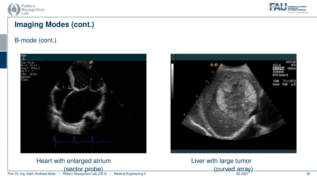
This is again the heart and this is one with an enlarged atrium. So you can see the heart valves here and then you see that this is the aorta coming in and this is the enlarged atrium. But you can also image the liver and here’s a large tumor. So this is the entire liver and you can see that there is this tumor in here which is probably not very good for the patient. 

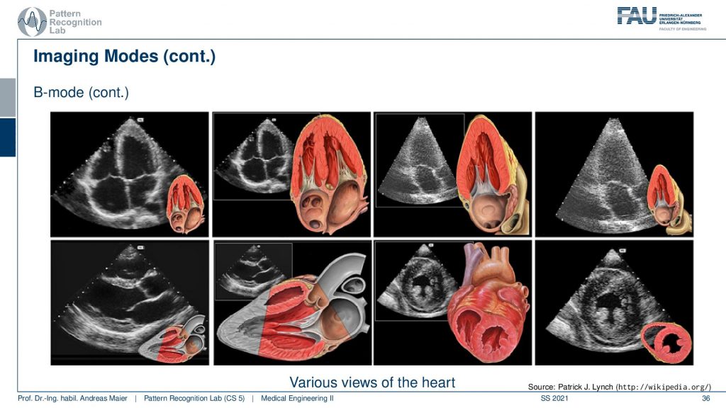
So of course, we can also see a couple of more images of the heart, and here for simplification we show a cross-section through an anatomic model and hear the respective ultrasound image. And if you’re able to build this in your head then you can also much more easily identify things on the ultrasound image. So here you see then this part being scanned and these are the respective heart chambers and here you see a different cross-sectional view and this is the part where we’re looking at. So if you know the heart by heart then you will be able to understand these ultrasound images much easier. Therefore it’s also very important that you know how you have been moving the ultrasound probe because when you don’t know where the ultrasound probe is facing, then you have a hard time interpreting those images. 

Then let’s go to the M-mode the motion mode.

In the motion mode. You essentially acquire many A-mode images over time and then you can visualize motion in a single image. The typical application is the cardio analysis and here you can essentially investigate the wall movement and here you see one of those M-mode images. 

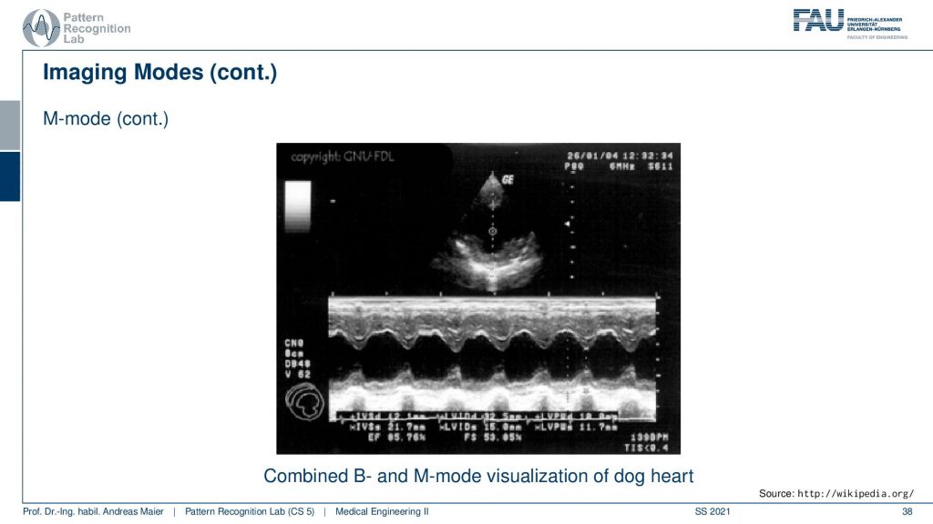
So here is a B-mode image and this is not the M-mode but then you can take one line in the B-mode image and plot it over time. Then you can see how the hard is beating and you can analyze for example whether there is a complete closure or not or, whether the corresponding points are in synchrony or not and you can diagnose this in order to find any abnormalities in the motion of the heart. So that’s also quite commonly being used. A last kind of mode that I want to introduce is the Doppler ultrasonography and here we use essentially the doppler acoustic Doppler effect to visualize the blood flow. 

The velocity and there are two different modes the Continuous-wave and the Pulsed wave. But all of this makes use of the doppler effect. Now how does this work?

Well, there’s the Doppler effect and there is a change in wave frequency relative movement which is causing this between source and observer. So if you have something that moves towards you, there is a frequency shift and if you have something that moves away from you there’s also a frequency shift. All of you probably know that from an ambulance car passing by with a loud siren. So you can hear a difference in frequency when it’s approaching you and when it’s heading away from you. This siren here is very classical and also in astronomy, you have this redshift where you can then also estimate velocities in interstellar configurations and here we want to use it for blood flow. 

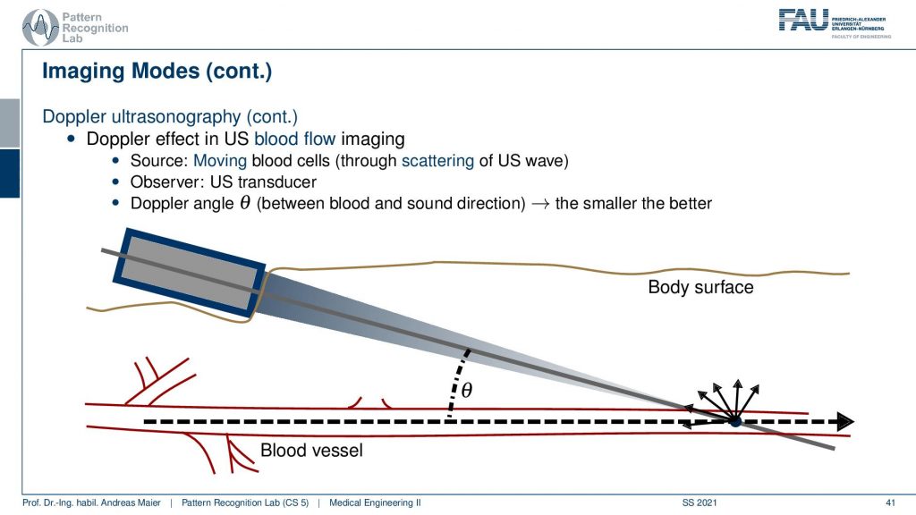
So the idea is then that you move the transducer at a very steep angle because you want to observe the flow. So you have to be seeing essentially particles almost in the view direction. Otherwise, there’s no Doppler effect. So you want to keep this angle low and then you can look at the blood vessel and dependent on whether the flow is going this way or this way you will observe a different frequency. This change in frequency that is caused by the actual reflection will then tell you in which direction the particles are flowing. So this is actually the acoustic Doppler effect and how it emerges here. Then there is also a couple of different kinds of application. 

So use a spectral doppler that visualizes the spectrum of the blood speeds. So you can simultaneously summarize this in the spectrum and then you see the kind of distribution of the speeds or, you use the color doppler where you color code and overlay on top of the B-mode image in order to understand in which direction the blood is flowing. You see here the distribution of the sound speeds. 

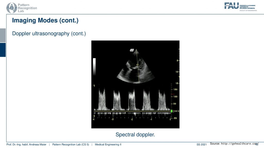
So this is the kind of spectral Doppler that we see here and you’ve probably also seen these kinds of colorful images here.

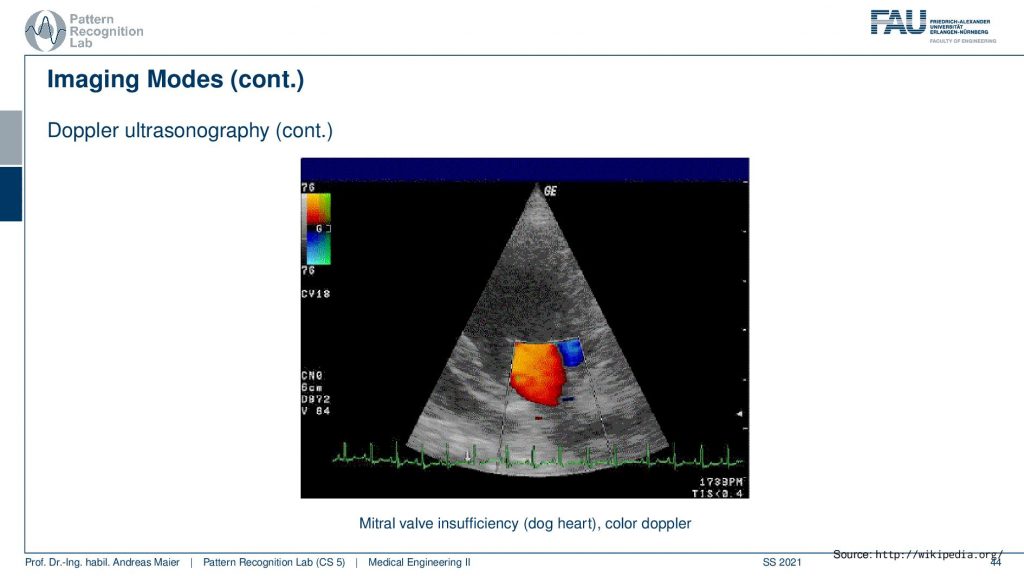
This is now the Mitral valve of a dog heart actually and you see the color Doppler effect here. So you see whether it’s blue or red that indicates the direction of the flow in that particular image. 

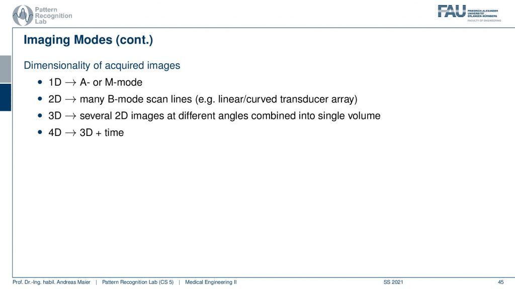
Well, let’s summarize this the 1D acquisition is the A or, M-mode. Then there’s the 2D acquisition that gives rise to the B-mode. Then you can also scan many B-mode images that give then rise to 3D ultrasound. If you construct the transducer in a specific way you can also directly acquire 3d volumes. So we’ve seen that in the image of the fetus in the mother’s womb. Of course, you can also do that in fast repetition. This then gives rise to 4D imaging. So these are the different imaging modes and of course, all of this is being used in clinical practice. Of course, a couple of words also on safety and ultrasound imaging.

This is already one of the last couple of remarks that I want to make. Ultrasound waves are not ionizing. So they are generally much safer but they can still harm the body. There’s the heating that is caused by the absorption. There is also another effect called cavitation. Cavitation can cause emerging gas bubbles in low-pressure phases of the sound wave and then you have to collapse at the high-pressure phase and this produces bubbles and this is not good. If you have cavitation you can introduce gas and gas for example inside blood vessels is probably not such a great idea. Technically this can happen for medical diagnostics. It’s rather low. So typically ultrasound is determined as harmless. It is even used during pregnancy. So it’s a mostly harmless kind of technology. So the therapeutical use of ultrasound is a bit of a different game. There you can break up gallstones and kidney stones and you can also use heat to destroy diseased or cancerous tissues. There the safety is also a probable concern and you have to make sure that you don’t cause any gas bubbles or that you don’t burn the wrong tissues. So this can also be done with ultrasound. 

Very well! This already brings us to the end of this video. So now you’ve understood ultrasound. You understood the properties of sound waves. How they propagate in tissues. How the density is relevant for sound speed and how the different acoustic impedances of tissues steer the reflection of sound waves. We’ve seen why we need this gel. We’ve seen the different configurations of the transducers. We use the piezoelectric effect in order to generate these high-frequency sound waves. We’ve seen the dependency of the frequency on acoustic absorption. So the higher the frequency the higher the absorption and this then also guides the penetration depth and in the end, we’ve seen a couple of applications on how we can use this to look at different parts of the body and how we can also interpret some of these ultrasound images. In particular, if you have good knowledge of anatomy you will be able to guide the view very quickly. So this is also a thing that requires quite a bit of training. A good ultrasonographer is also able to create very reproducible angles and can make the same images over and over again. But of course, you have to have the right experience. If you’re not very experienced, you will always get oblique angles between the different acquisitions. Then all the measurements are much more difficult because it of course makes it different if you measure something in a different plane in a different intersection plane. So this is also why ultrasound is typically called a subjective imaging modality because all of the measurements and the accuracy of the measurements depend on the experience of the actual user.  This already is the end of this video. So I hope you enjoyed this video again and I’m very much looking forward to seeing you also in the last video of this lecture. This is going to be the optical coherence tomography again something that is based on wave propagation but this time at a much finer scale than ultrasound. Thank you very much for watching and bye-bye.

If you liked this post, you can find more essays here, more educational material on Machine Learning here, or have a look at our Deep Learning Lecture. I would also appreciate a follow on YouTube, Twitter, Facebook, or LinkedIn in case you want to be informed about more essays, videos, and research in the future. This article is released under the Creative Commons 4.0 Attribution License and can be reprinted and modified if referenced. If you are interested in generating transcripts from video lectures try AutoBlog

References   

• Maier, A., Steidl, S., Christlein, V., Hornegger, J. Medical Imaging Systems – An Introductory Guide, Springer, Cham, 2018, ISBN 978-3-319-96520-8, Open Access at Springer Link

Video References

1. Sonosite Cardiac Ultrasound https://youtu.be/H_3V9xlDMA0
2. Baby Driving https://youtu.be/8j8iXYRWfyg
3. Wireless Handheld Ultrasound https://youtu.be/Qzowd0y4hZU

Kategorie: Lecture Notes in Medical Engineering