Optical Coherence Tomography

These are the lecture notes for FAU’s YouTube Lecture “Medical Engineering“. This is a full transcript of the lecture video & matching slides. We hope, you enjoy this as much as the videos. Of course, this transcript was created with deep learning techniques largely automatically and only minor manual modifications were performed. Try it yourself! If you spot mistakes, please let us know!

Welcome back to Medical Engineering. This is already the last video of our lecture series and today we want to discuss optical coherence tomography. So this is an imaging modality that now also uses light as a wave. You’ll see that we are actually using it in a very similar setup to ultrasound but this time we’re operating at very different wavelengths. Yet you can see that the emerging images and also image formation is very similar to ultrasound. So looking forward to exploring optical coherence tomography with you guys. 

We will start with a short introduction. 

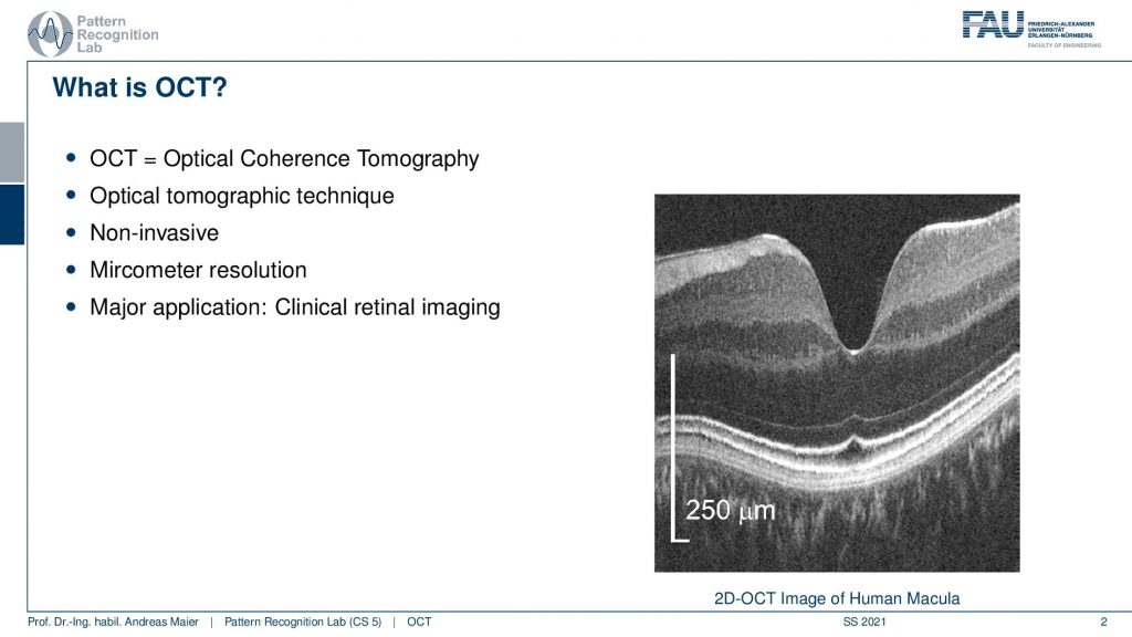
So OCT is again a tomographic technique. So we produce again slice images. It’s non-invasive and operates at micrometer resolution. The major applications are clinical retinal imaging. So we are in ophthalmology the science of the eye and the treatment of the eye. You can already see here, this is a 2D OCT image of the human macula. So this is the background of the eye and you can see here that 250-micrometer resolution is this long in this direction and this long in this direction. So it’s an anisotropic image that we see here and the scales are much longer along the y-direction than on the x-direction here. So what you see here is the background of the eye. So this is the Macula and you can see here that there are different layers in the retina. We can see how these layers actually are fused together here and you can very nicely analyze the structure of the retina with this kind of image. If there were any kind of pathologies you could see that in these images. Now let’s think a bit about why this is an important modality. 

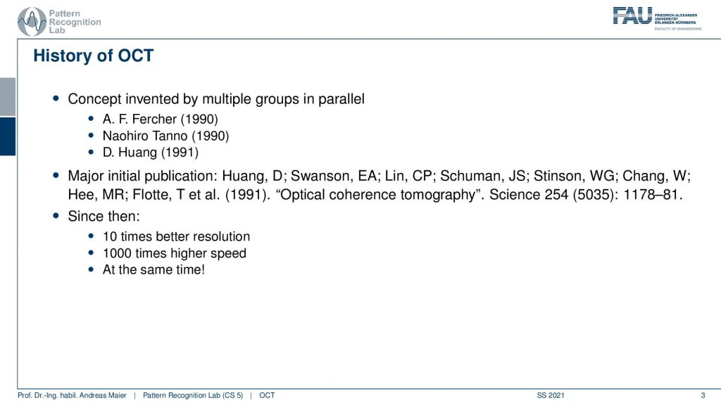
So this concept has been invented by multiple groups in parallel by Fercher, Tanno, and Huang. You see that the publication dates are almost in the same year. The major initial publication was done by Huang and this is called “Optical Clearance Tomography” and it appeared in science has been cited many thousand times and since then in 1991 we have 10 times better resolution a thousand times higher speed and this all at the same time. So there has been also quite some progress over the past years since the original publication. 

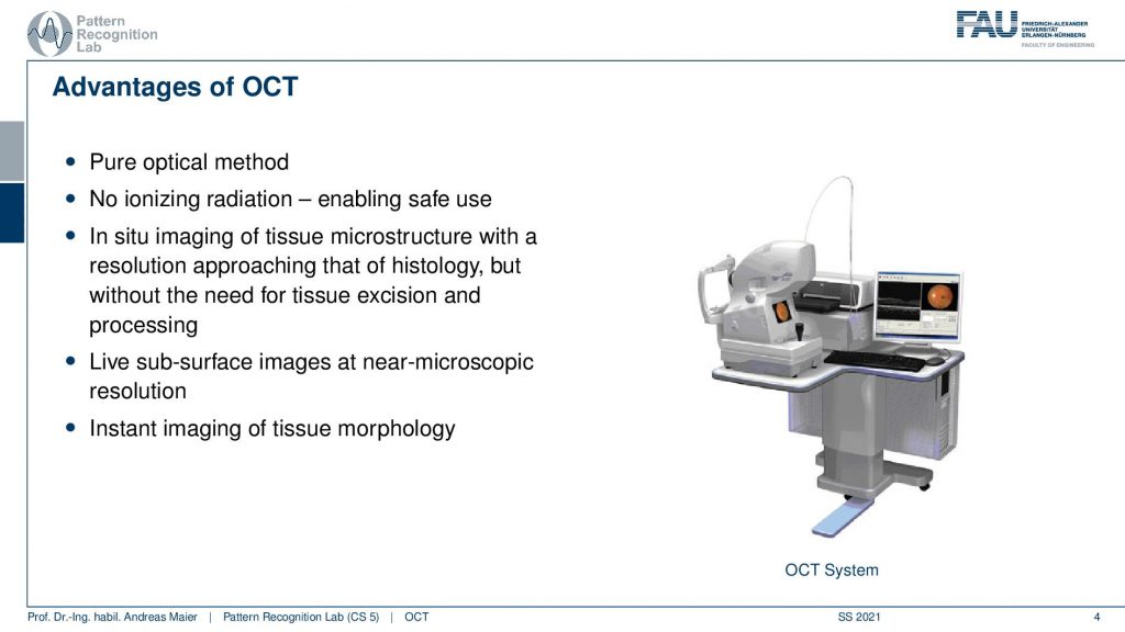
Now let’s have a look at the advantages of OCT. It’s a purely optical method. There is no ionizing radiation. This is essentially all-optical light and close to optical light. So it’s safe for use. You do in situ imaging so you directly image the tissue. You don’t have to operate on the eye to extract any tissue or something like that and you can get the microstructure at a very high resolution. It also allows for live subsurface images at near-microscopic resolution and it’s an instant technique for imaging the tissue morphology. Here you see an OCT system this is typically where the patient moves his head. Then the operator uses the small stick in order to move the kind of imaging device here such that it’s aligned with the optical axis of the eye and then you can scan directly the retina. So this is how the system looks like and you can see that there is also a certain regime where OCT is operating. 

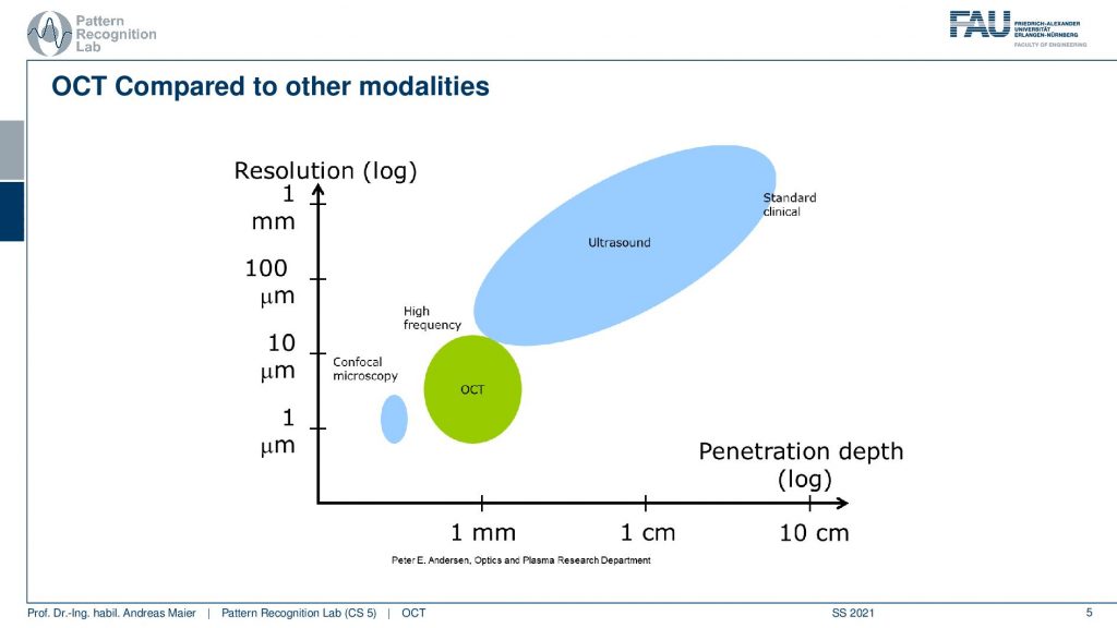
You can see that ultrasound is essentially here and it has penetration depth from millimeters to centimeters even beyond centimeters. OCT is operating here. This is the part where OCT is operating. Here we are in the resolution ranges between 10 and 1 micrometer and we are in the penetration depth below one millimeter approximately one millimeter. So we can’t image very deep into the tissue. You can see that here, is also confocal microscopy. So in microscopy, we take out the tissues and there we have very low penetration depth but very high resolution. So we are essentially in a similar regime as microscopy. 

The working principle of OCT is done on several scales. So we start with a high-level overview. Then we talk a bit about light as a wave and the interference and this will then give rise to the actual imaging technique. So let’s start with the high-level overview.

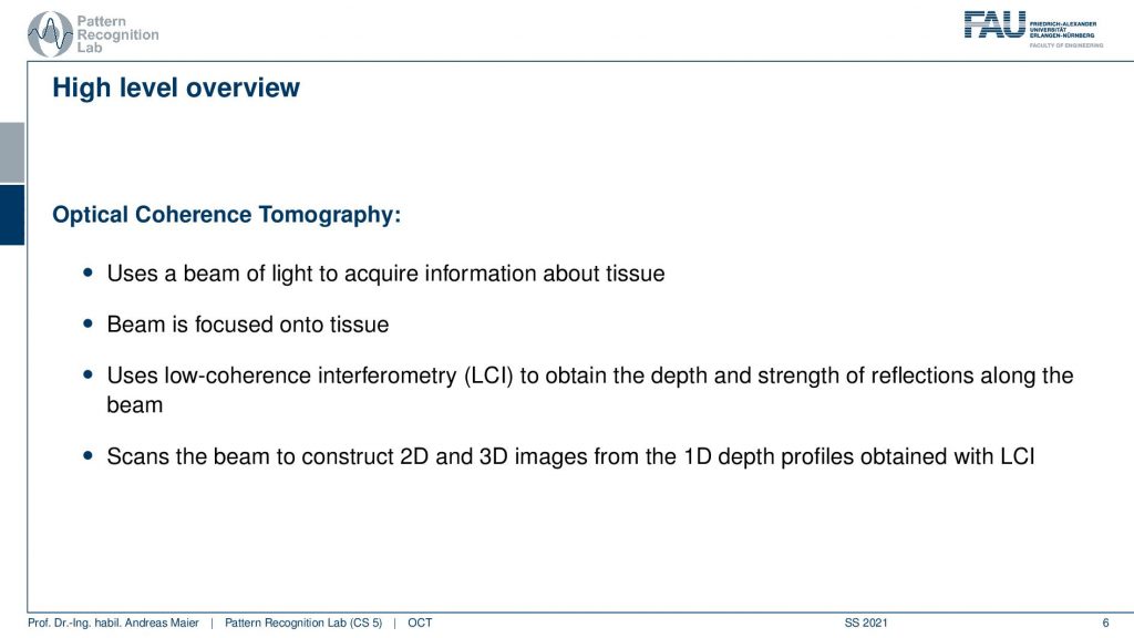
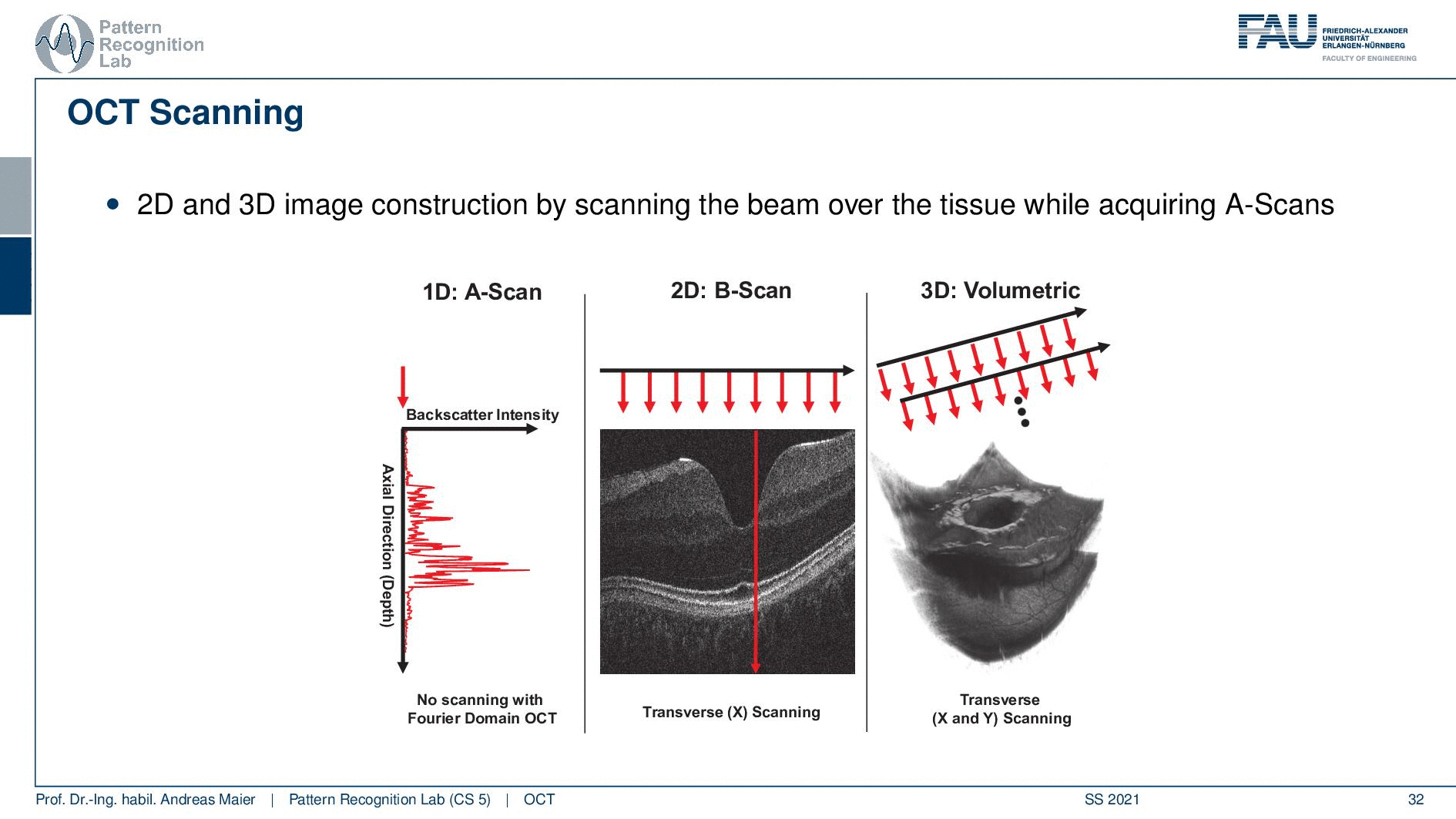
OCT uses a beam of light to acquire information about the tissues. The beam is focused onto the tissue and then we use low coherence interferometry LCI to obtain the depth and strength of reflections along the beam. So again we have essentially the reflections along the beam very similar to ultrasound and then we scan and reconstruct 2D or 3D images from 1D depth profile. So here the concept of the A-scan and B-scan will come again because we’re essentially scanning single depth profiles and then assemble different images from that. 

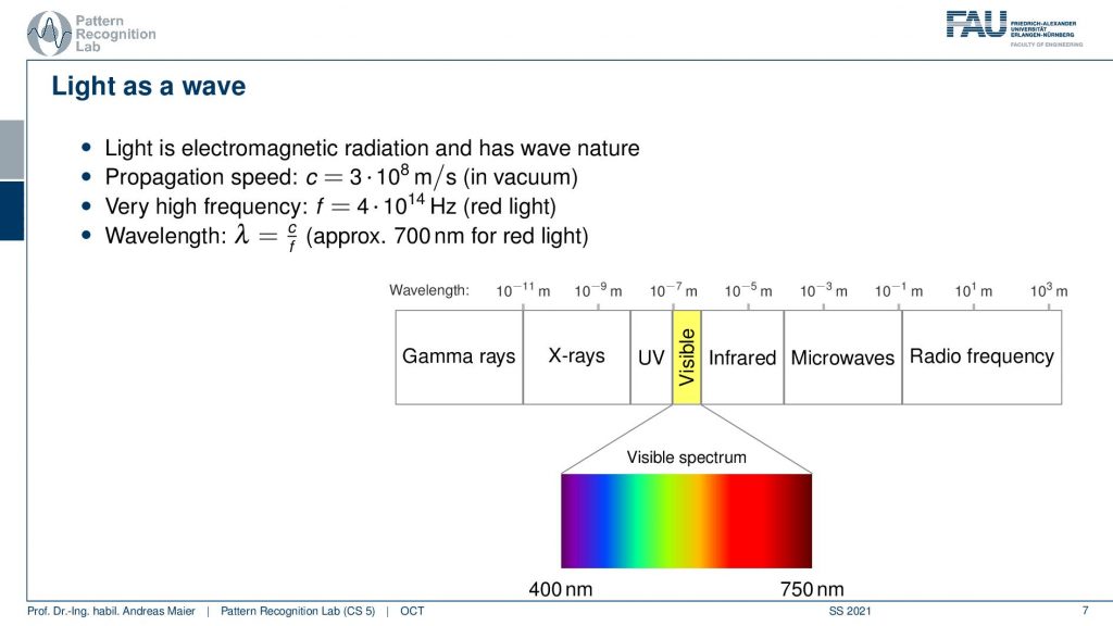
Now we use light as a wave and the kind of light that we want to use is essentially here in the range of the visible light. You’ve heard about this many times in this lecture. You already know the electromagnetic spectrum and now we’re very close to visible light or working with visible light. 

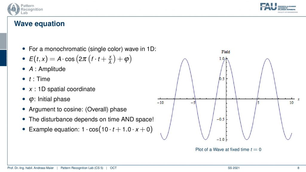
The light propagates with the wave equation we have an amplitude. We have the time and this can be put together in this wave equation. Here then we have an initial phase and the 1D spatial coordinate and this allows us to describe a wave over time and how it propagates. So the disturbances that we’re interested in depending on time and space. This is again a wave and we have to see how we can model this here. 

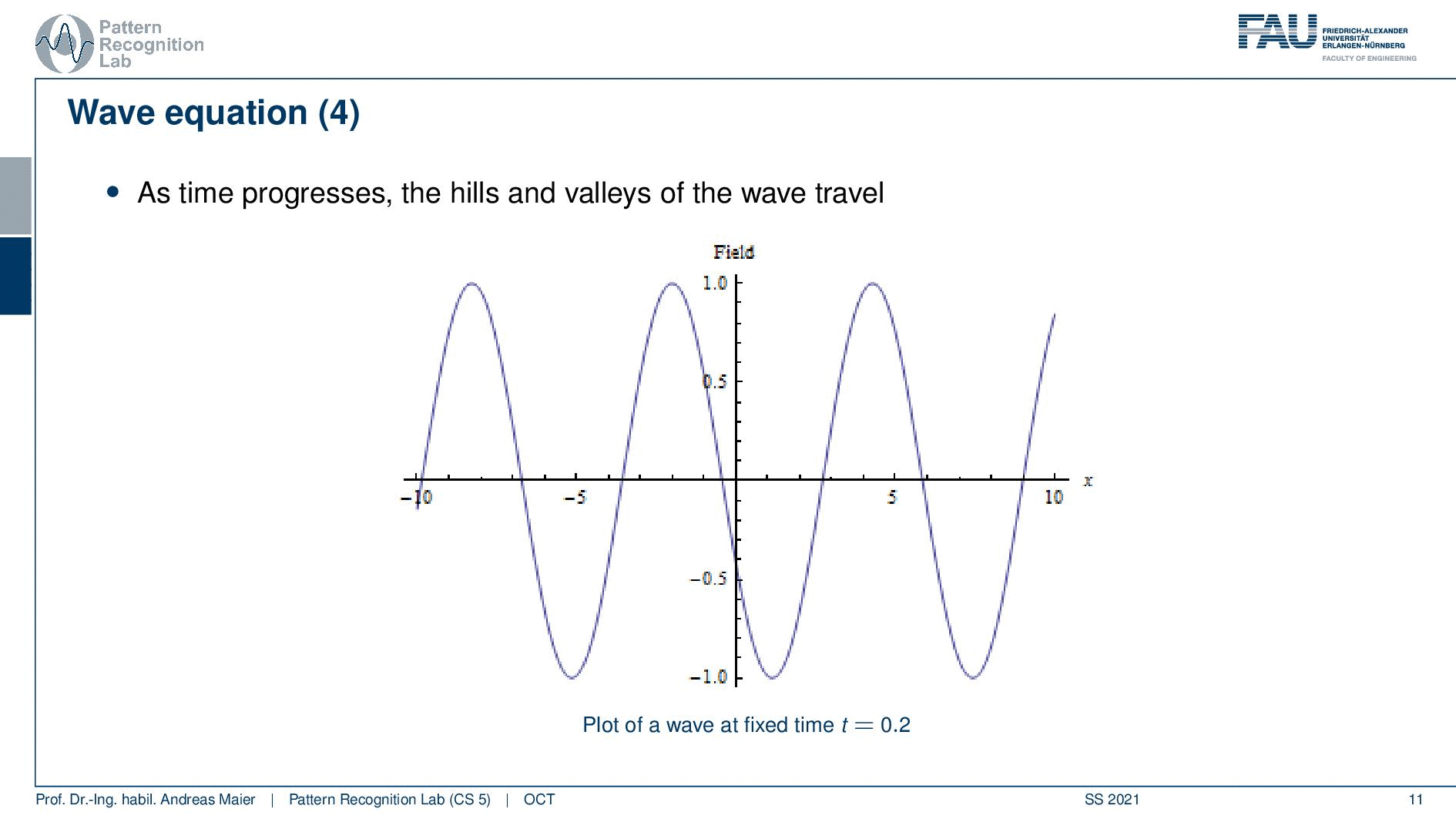
So what we do in the following is we essentially think about this wave and you can see now if I change the time the wave changes and propagates through our space. This is essentially corresponding to a shift here in our wave. 

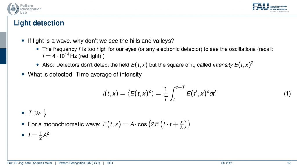
Now if we want to detect this wave what is happening is that we are computing something like a time-averaged intensity. This is typically computed as an integral over the observed function e. So this amplitude to the power of 2 and this is the actual measurement. For monochromatic waves, we can express this as the amplitude times this cosine expression here. Therefore the intensity is then simply determined as 1 over 2 times the amplitude squared because we have this time integration here and obviously the time is also much longer than the wavelength for our integration. This means we just see this average effect here. 

Let’s talk a bit about interference and in interference, we need multiple waves. We already heard about that. So we have wave one, wave two,……, wave n, and the net field. So the total composition of all the waves is given as a sum over all the waves and this is the overall field. Then we can measure the overall field in some detectors. This leads to interference because now we have different waves and they’re superimposed. This then causes a change in the total field and now we’re unfortunately not detecting the field but only the time-averaged intensity and that makes things a little bit more complicated. 

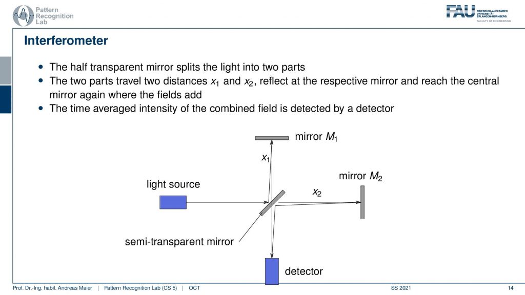
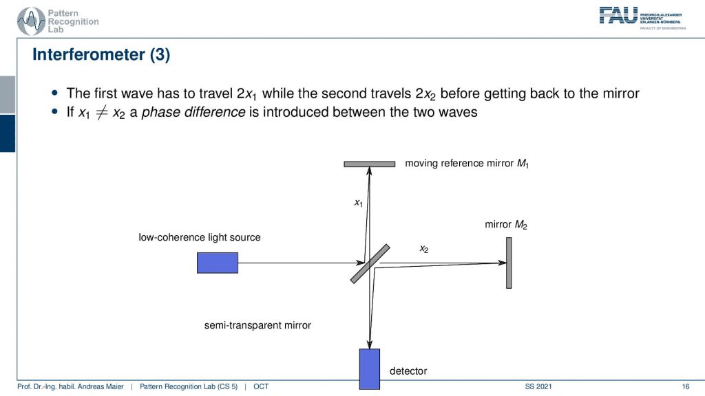
So this then gives rise to another interferometer and we’ve already seen a similar kind of concept when we are talking about differential phase-contrast imaging. This is done here again by using different waves, but we are now using mirrors in order to create the interference. So we have first a half-transparent mirror. This is a semi-transparent mirror and there we have a light source. So the light goes through here. Then it gets reflected and a part is being reflected into here and another branch here is reflected to up here and here it also gets reflected. So this constellation here then allows us to detect something down here. This is essentially measuring the interference between the green path and the red path that I’ve been just drawing. This essentially allows us to construct an interference with the beam itself. Now depending on the distances x₂ and x_1, I will get a different interference pattern and as we discussed already previously. If I just have one wavelength then I’m able to construct essentially a stable interference. I could by moving these mirrors construct these different fringe patterns. So the time average intensity is then combined here in the detector and I can essentially then determine either whether we have a stable constructive interference or, canceling and the destructive interference. This all depends on the configuration of x₁ and x₂.

So how can we use that?

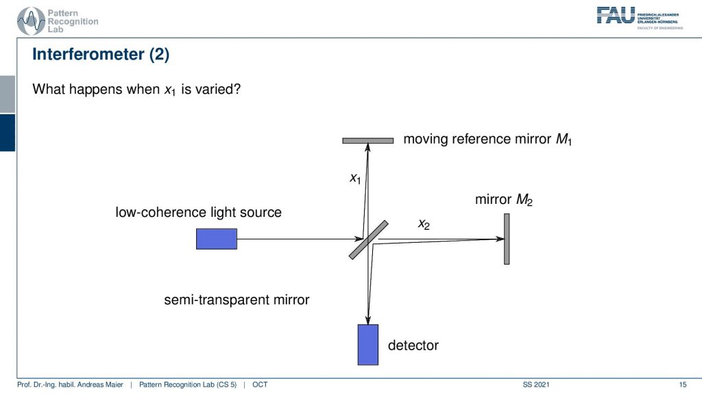
 Well, we can now use a moving reference mirror and we are changing the distance in x₁. If I do that I can analyze now what’s happening at mirror 2 and I can change how the interference pattern here changes. So that’s actually pretty cool and I could now work with the interference patterns. But the problem with that is all that I can differentiate happens within one wavelength after one wavelength everything is repeated. It’s not that great because then we can only resolve exactly one wavelength along with our investigation. So that’s not that great right. 

So we can now of course move everything back and forth but everything that we can analyze has to lie within one wavelength. If I go one wavelength further the same pattern will just emerge again and there is no additional benefit that is produced by this. So that’s not so great.

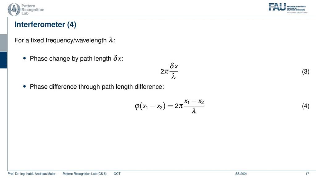
So for a fixed frequency wavelength then I essentially can only reconstruct the differential phase here and we have the same fringe patterns popping up again. We only get the contrast friends between essentially two maxima of the fringes and this is the whole analysis window. So we’re kind of stuck in this position. 

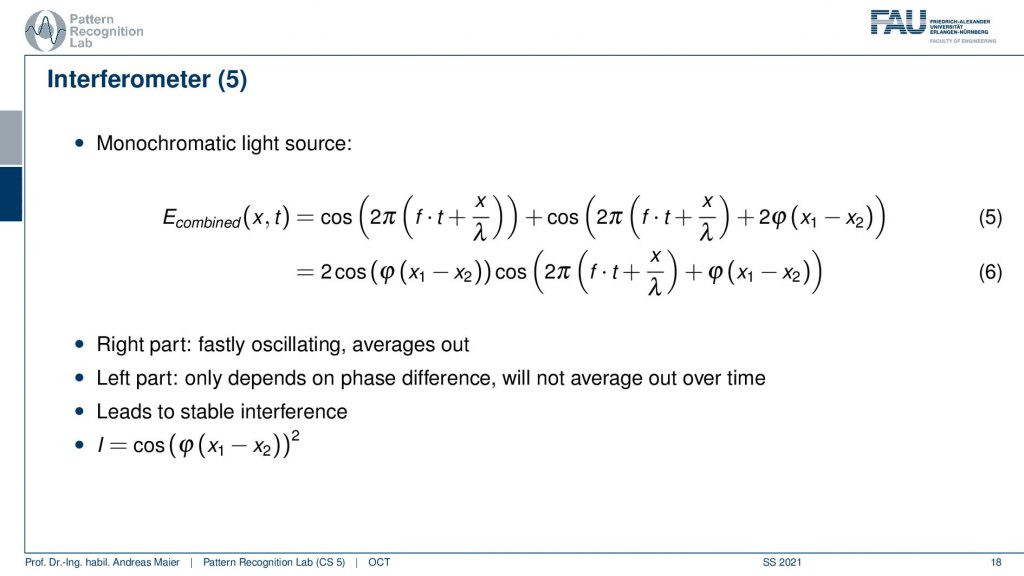
So maybe the monochromatic light source is not such a great idea after all because then we have stable interference and we can’t get any additional kind of resolution. 

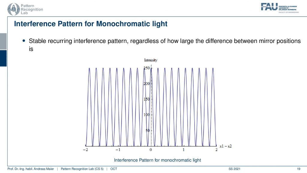
So let’s go ahead and see what happens if we use the monochromatic light source. So you see the stable interference and everything that we can essentially analyze is between one of those wavelengths. Then we repeat it again and again and again. So that’s not that great. So we have to somehow work with a different kind of option and this is done by mixing more waves. 

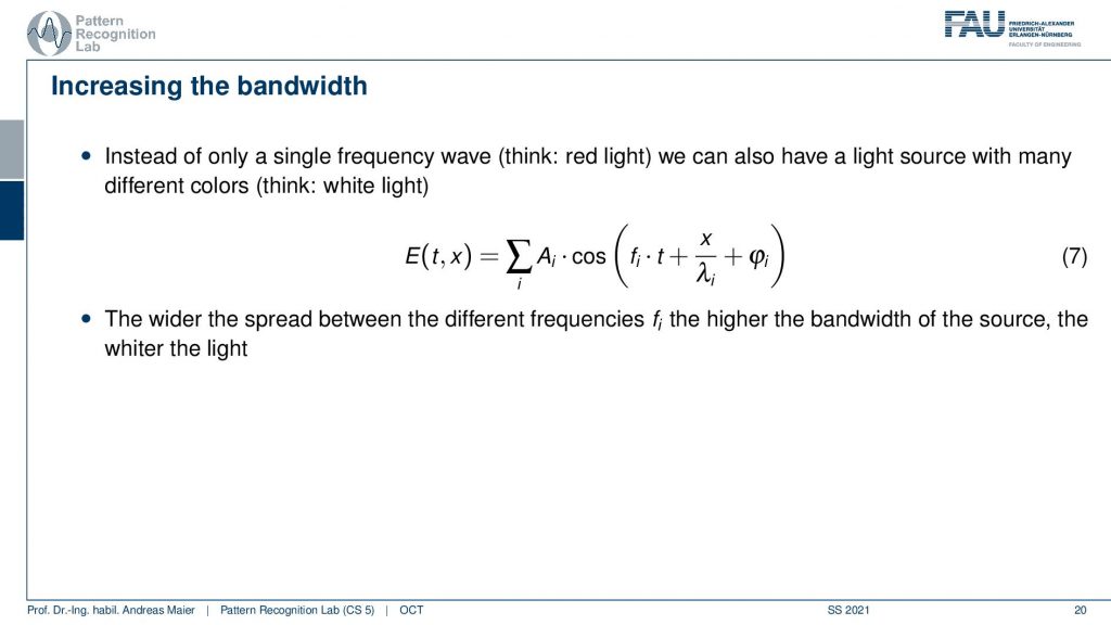
So now we sum over a different set of waves and this is then also known as increasing the bandwidth. So the wider the spread between the different frequencies is the higher the bandwidth of the source and the wider the light. So essentially if we compose many kinds of frequencies we get a whiter light. So why would we want to do that?

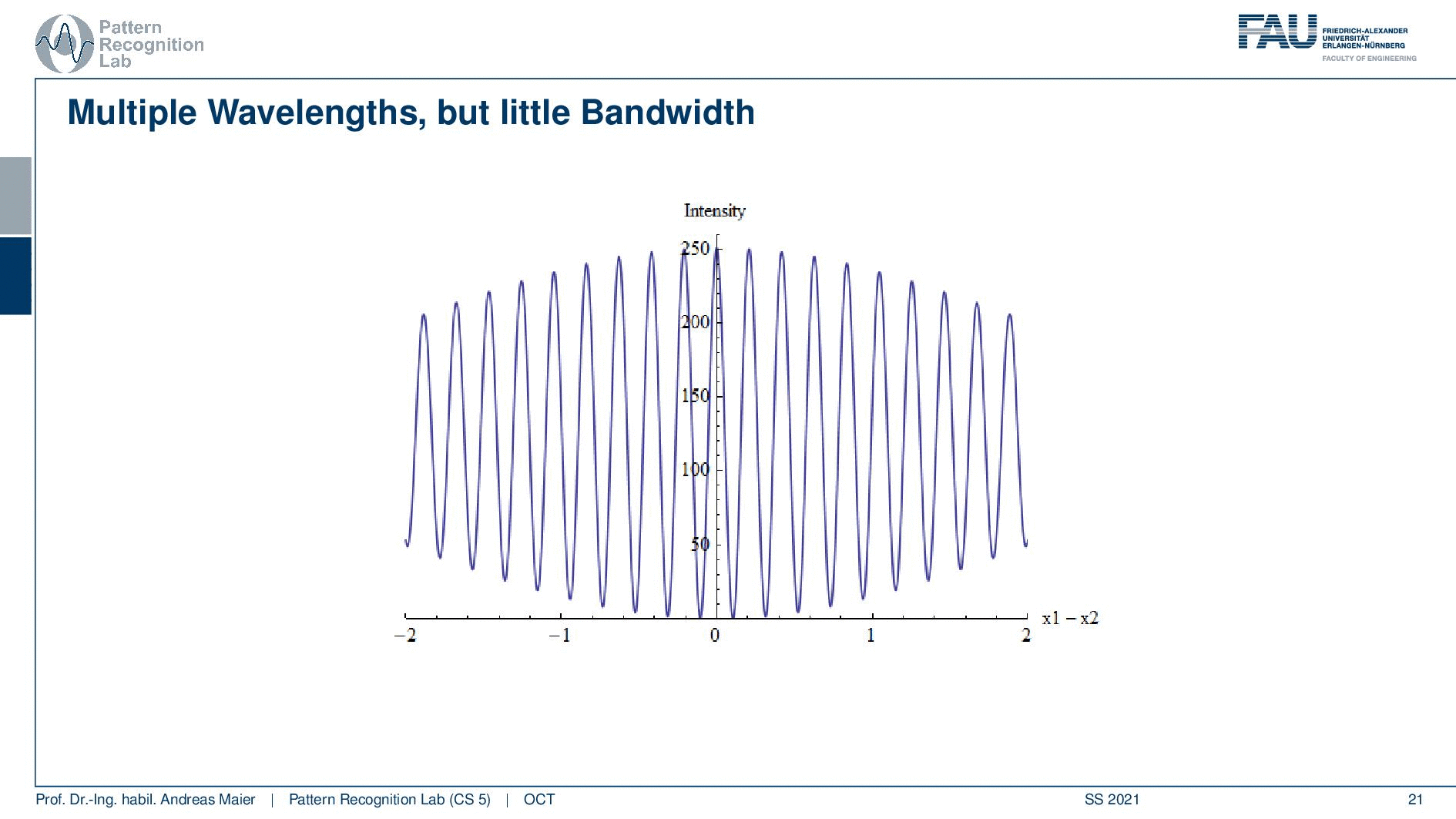
Well, let’s have a look at a signal with multiple wavelengths but little bandwidth. Then the intensity propagation looks like this. Now let’s increase the bandwidth. We double it and we double it again and we can double it again and what you see is that we somehow reconstruct a kind of pulse. We get a pulsing here and the more bandwidth we increase the more our pulse gets localized and this localization is pretty good. If we include essentially all of the frequencies we probably end up with a Dirac pulse because the Dirac pulse contains all of the frequencies. So you see something similar emerging here.

Here we then observe that the higher the bandwidth of the source the sooner the interference vanishes. This also then gives rise to the so-called coherence length which is the maximum difference in mirror positions for which we can still see the interference. So the coherence length essentially tells us how far the interference pattern still is working. So for monochromatic light, the coherence length is infinite. If I only have a single wavelength I have an infinite coherence length. So I can move the mirror everywhere and I always get the kind of inference pattern but it’s repeating all the time. Now if I have more different frequencies the shorter the coherence length. So I have a shorter effect of this interference pattern but I also get a shorter pulse. So for a light source with short coherence length, we will only see oscillations if the parts are closely matched. So this is something we can now use and this brings us then to the following setup. 

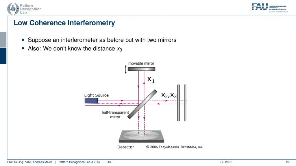
So let’s suppose an interferometer as before but now we have two mirrors and we have the mirror x₂ and x₃. So there are two mirrors here we have again the light source and we don’t know the distance x₃ but we have the movable mirror here and the detector down here. Now we can of course use the same kind of setup and we can move the mirror up and down.

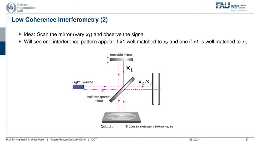
Now what happens is that if I vary our mirror one at a certain coherence length at a certain position, I will get this interference pattern. Then I sum up all of the waves. So we will only get the intensity of the interference pattern but this means I just get a signal. Again we essentially suffer from this problem that we are not measuring the wave directly but only the integration. You remember we had a face-stepping grating in the phase-contrast image. But here we are just integrating over everything but we just get a signal at the right depth. So we essentially use the interference pattern now only to determine whether a signal is present or not. This way by moving the mirror up and down, if I have it at the right position of x₂ I get interference and if I have it at the position of x₃ I get an interference. This will essentially then cause a signal in the detector. Now by moving our x₁ back and forth and then I will get essentially an interference pattern here at x₂ and another interference pattern here at x₃. So there’s of course a little bit more oscillation but I get pretty clear peaks at the positions x₂ and at the position x₃ if I vary this movable mirror here. Now you see how I can detect essentially reflections back in the back of the eye by moving this mirror here. So that’s the main idea. 

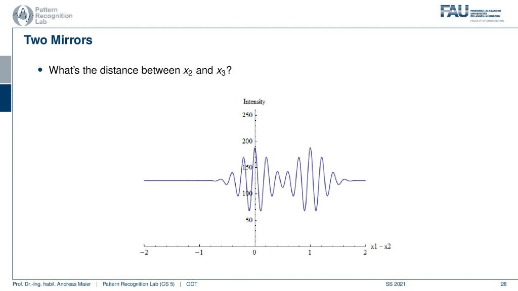
Now of course the distance matters and the distance is governed by the coherence length. So if I have a rather long coherence length like in this example it may be difficult to differentiate the two signals. 

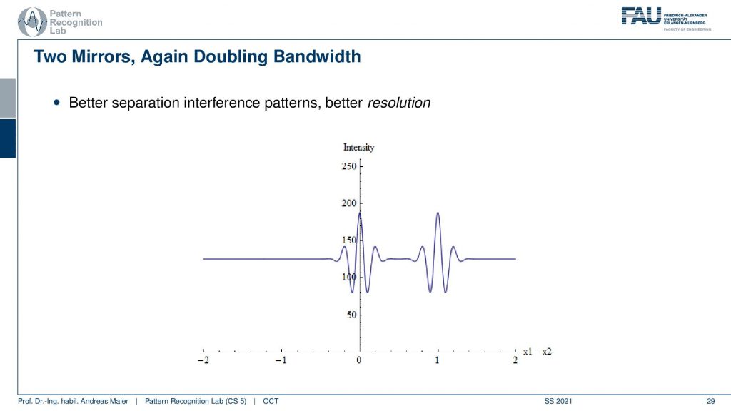
But if I have a shorter coherence length then I can separate the two signals better. So here we again double the bandwidth and then we have better separation and a better spatial resolution in our scanning approach. 

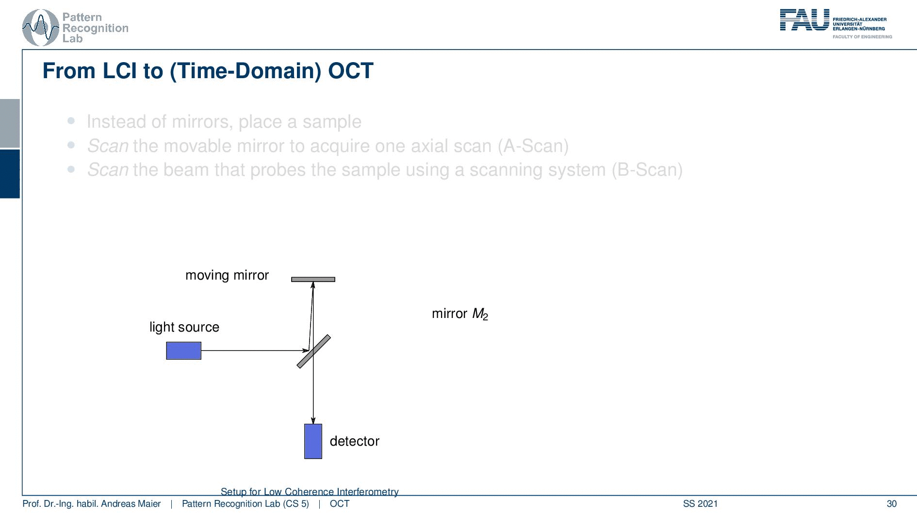
Well, now we can go from the actual time-domain OCT to a different kind of setup and there we don’t have a mirror anymore but instead, we have a sample. So here you could say that we place maybe the eye and then we are interested in scanning the retina back here. We can have again this movable mirror. So this again then allows us to determine the reflections in the back of the eye. Now we can move the mirror up and down and this constructs an A-scan. So this gives us a depth profile along the retinal depth direction. Then we can scan many of those beams in this direction. Then we get a B-scan. So you see this is already an image and we can even repeat that and then we could scan an entire volume. So this is how we get a time domain scan over an entire volume. So this takes a little longer. It’s not so efficient. 

This is why there is the so-called Fourier domain OCT and here you use a fixed mirror. This is a sample this is the eye and now we use a spectrometer here. So we analyze the single pulse that we send in here. We analyzed the spectrum and from that, we can measure one A-scan with a single spectrum measurement. This then allows us to do much faster scanning. So if you had a thousand steps for the A-scan and you can measure a thousand values at once with the spectrometer, then you have a speedup of a factor of 1000. So this is then the A-scan and we still have to perform a Fourier transform. Because we’re actually acquiring the Fourier transform of the desired A-scan, we have to convert it back to the spatial domain. But then we have much higher speed and even better sensitivity and also what’s cool is. there are no mechanical moving parts. So we also have a more robust system. So nowadays the Fourier domain OCT is being used and then you essentially get the difference here. This is the classical A-scan where you have to move this kind of mirror and you can see here this is the profile and with Fourier OCT there is no additional scanning required. So you just instantaneously get the entire A-scan in a single shot. 

Then we can summarize essentially what we’re doing in OCT there is the A-scan the B-scan and the volumetric acquisitions that allow us to scan entire 3D volumes of the back of the retina. So this is cool technology and it allows us to see in vivo 3D resolved high-resolution images of the background of the eye. So that’s a really cool technology and people are still working on this to improve the kind of acquisition technology. 

Now let’s look at a couple of applications and obviously the first and foremost application is in ophthalmology. 

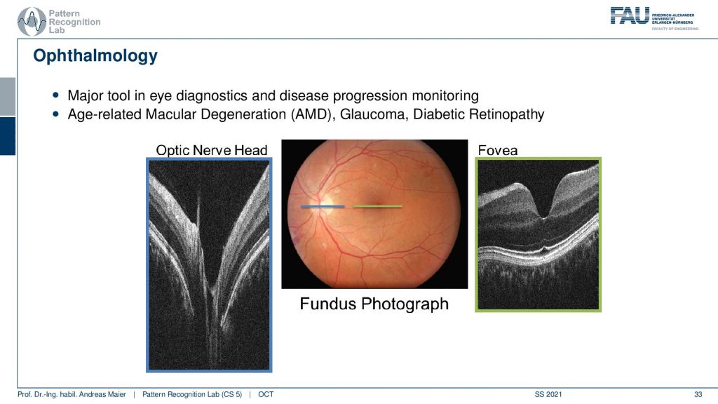
So here you see a couple of images. This is the so-called optic nerve head and this is the area where all of the blood vessels penetrate the retina and essentially supply all of the retinae with blood such that the nerve cells can function really well. You can also see that here in green this is the Fovea. The fovea is the region where you have the highest sensitivity. So the optic nerve head is also known as a blind spot because there you essentially only have blood vessels but nothing that actually perceives. The fovea is the area where you have the highest resolution and this is what you always try to focus on. We actually also see that there is a varying resolution on your retina where you have the highest image resolution here. Then you have thicker blood vessels here in the outskirts which then also diminishes the resolution of your eye in this area. So we move the eye all the time in order to make sure that the highest resolving area is always focusing at the object that we currently have our attention on. In our brain, we are reconstructing images that look really highly resolved and we never notice that we actually have a pretty poor resolution in this area of the retina. So, of course, those two areas are highly relevant to diagnose different atomic diseases and this is for example associated with diabetes, and also actually the retina is a part of the brain. So you can also identify the early onset of certain neurodegenerative diseases in the retina. So that’s a very interesting approach that we can also find early onsets of dementia in certain areas of the retina. So this is interesting then there are of course a couple more example images. 

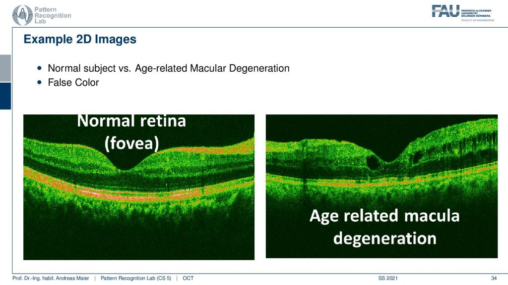
So here you see a normal phobia and we have this nice color coding and this is an age-related molecular degeneration. Here you see suddenly these holes here popping up. You also see this vessel shadow but here you see that this is not the youngest kind of retinal structure. This can then also lead to certain ophthalmic diseases and then also a loss of actual visual acuity. 

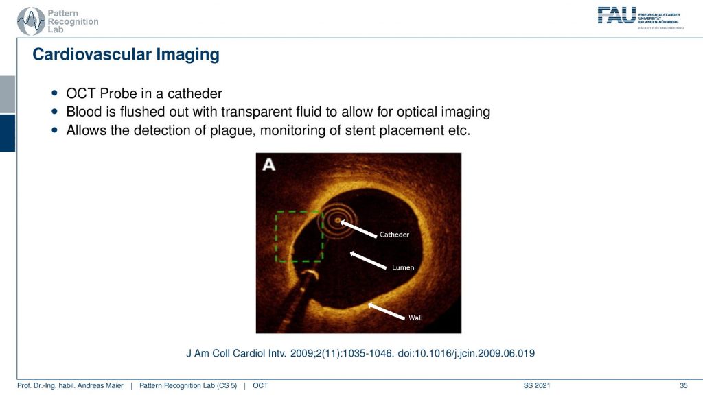
There’s also cardiovascular imaging. So we are not just using this at the eye, you can also augment this on a catheter and then you can scan the vessel wall and it allows us essentially to analyze for example plugs and the wall of vessels. So this is also an important technology where OCT comes in very handy. The last application that I want to show is a pretty cool one. 

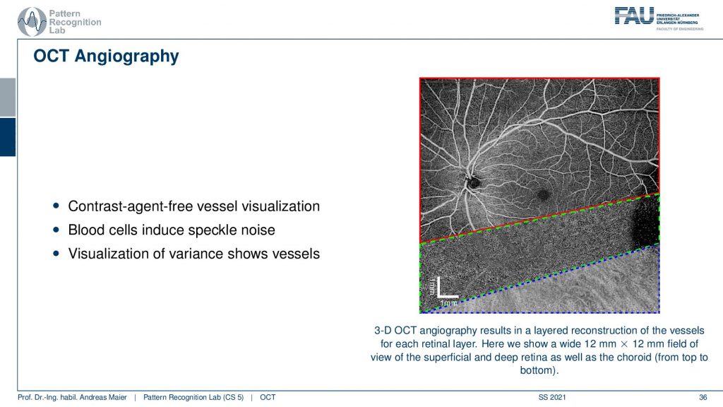
This is called OCT Angiography and you remember that we have this speckle-noise whenever we have structures that are approximately in the wavelength of our wave. This is also true in OCT. So what you can do is you can scan the retina multiple times and then do a noise analysis for every voxel and then project it. Then you can essentially summarize the different retinal layers, the projections and this allows you to get different images. Here you see essential the superficial layer and then the deeper layers. In the deeper layers, you can then visualize essentially repeating noise textures and the cool thing is because blood is approximately the same size as the wavelength of the waves that we are using here. So you get the speckle noise and then if you average this a little you get these wonderful vessel representations. Here you’re not using any tracer or contrast agent. You can just depict the vessels and the tracer are essentially the blood cells themselves. So wonderful technology contrast free and you can image very nicely the vessel structure of the eye. So, OCT optical coherence tomography angiography is a wonderful technique. 

Let’s conclude this a little bit. I have a couple of take-home messages for you. 

So optical coherence tomography allows in situ imaging. It has a high resolution and it’s non-invasive, it relies on light as a wave interference and coherence length, and the coherence then essentially then determines the resolution of the system. But the interference is the key component that actually allows us to determine whether there is a signal or not. It became really a standard in ophthalmology systems that are used over the entire globe and this technology is being used in standard clinical care. So this is really exciting technology and I’m very happy that we have good collaborations with other groups worldwide. We are also trying to push ahead of the state of the art in optical coherence tomography. 

I have some nice book chapters here again. This is from our textbook which you can download for free by the way. So it’s all creative commons open access and two more publications here that you can find on “Optical Coherence Tomography: Technology and Applications” as well as the “Optical coherence tomography: principles and applications”. 

So this already brings us to the end and now it’s actually the end of the entire lecture. So you’ve now seen essentially a broad overview of different medical imaging systems. We started with the motivation where we need them for many different diagnoses. Then we’ve seen that we actually went through the entire systems theory. The Fourier transform, linear systems theory, convolution, and so on. These are fundamental techniques that you need to understand actually the whole imaging system. We talked a bit about image processing and some simple image processing techniques. Then we started talking about different modalities starting with endoscopes, microscopes and then we went on into all the volumetric kinds of imaging modalities MR. We’ve seen X-rays, we’ve seen CT, we’ve seen the X-ray phase-contrast went on for the functional imaging where we had PET and SPECT. Then we investigated ultrasound and optical coherence tomography. So I hope you enjoyed this small lecture series. I think it’s a very good overview of the different technologies that are used in medical imaging systems. If you liked it please leave us with a like and tell people about this lecture. You can also see it completely free on youtube. So you don’t have to be a student of FAU to watch it and also all of the videos the slides and the script, the textbook is all open access. You can download everything for free and yeah you can also reuse them. It’s a CC by license. So if you’re writing your bachelor’s master’s thesis or any papers go ahead and just reuse the figures as long as you cite them I’m perfectly fine with that. Thank you very much for watching. I hope you enjoyed this small set of videos. If you like them please tell us, please tell the world, and maybe you attend another lecture of us at some point in time. We also have very nice lectures on machine learning. We also have lectures on deep learning and the newest trends. We are also working on various image processing computer vision, speech processing lectures that we will also produce in the same way with open access materials so that there are available to the entire world. Thank you very much for watching and bye-bye. 

If you liked this post, you can find more essays here, more educational material on Machine Learning here, or have a look at our Deep Learning Lecture. I would also appreciate a follow on YouTube, Twitter, Facebook, or LinkedIn in case you want to be informed about more essays, videos, and research in the future. This article is released under the Creative Commons 4.0 Attribution License and can be reprinted and modified if referenced. If you are interested in generating transcripts from video lectures try AutoBlog

References   

• Maier, A., Steidl, S., Christlein, V., Hornegger, J. Medical Imaging Systems – An Introductory Guide, Springer, Cham, 2018, ISBN 978-3-319-96520-8, Open Access at Springer Link

Video References

1. Interferometer Animation https://youtu.be/UA1qG7Fjc2A
2. OCT Angiography https://youtu.be/auSNvLRKJN0

Category: Lecture Notes in Medical Engineering