System Theory – Introduction to Sampling and Quantization

These are the lecture notes for FAU’s YouTube Lecture “Medical Engineering“. This is a full transcript of the lecture video & matching slides. We hope, you enjoy this as much as the videos. Of course, this transcript was created with deep learning techniques largely automatically and only minor manual modifications were performed. Try it yourself! If you spot mistakes, please let us know!

Welcome back to Medical Engineering: medical imaging systems and today we want to talk about another very very important concept and this is sampling and quantization. 

So this is the process that is involved to convert a signal from the analog domain into the digital domain. It is very important and you will see that everything we do in medical imaging systems as soon as it gets digital you have to know about the concepts of digitization and sampling quantization. So I hope you will enjoy the next couple of videos this won’t be too long of a video. It will have fundamental concepts that you really need to know about if you want to make a career in medical engineering and in particular you’re interested in digitization of any kind of signals.

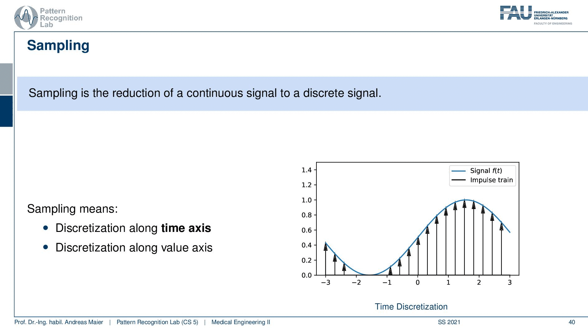
Sampling is the process of getting a signal essentially into a digital computer. So sampling is the reduction of a continuous signal onto a discrete signal. We want to do it in a way that we don’t lose any information. So this means that we have to discretize along the time axis. So this is shown here on the right-hand side. We have to essentially figure out the continuous signal at certain points. So these are indicated with the arrows here on the right-hand side. So we have to sample the signal at these time points and this is of course discrete because we cannot store infinitely many variables or observations in our computer. The other thing is we need to quantize and this means that we also have to assign discrete values on the value axis. So we cannot just save infinitely many values in our computer. So we also have to have a step size here in the quantization. This is the main problem of sampling and digitization. The key problem that we’re actually facing is how do we select the parameters essentially the step size in between the samples and the step size in between the value such that we don’t lose any information. On the other hand, we also want to be able to use as little space as required. So we don’t want to have excessively many of these sampling steps because if I have to sample twice as often I need twice as much space. I also need to process twice as much data. So this is really crucial to set these spacings here correctly such that nothing really goes wrong. Things can go wrong quite a bit.

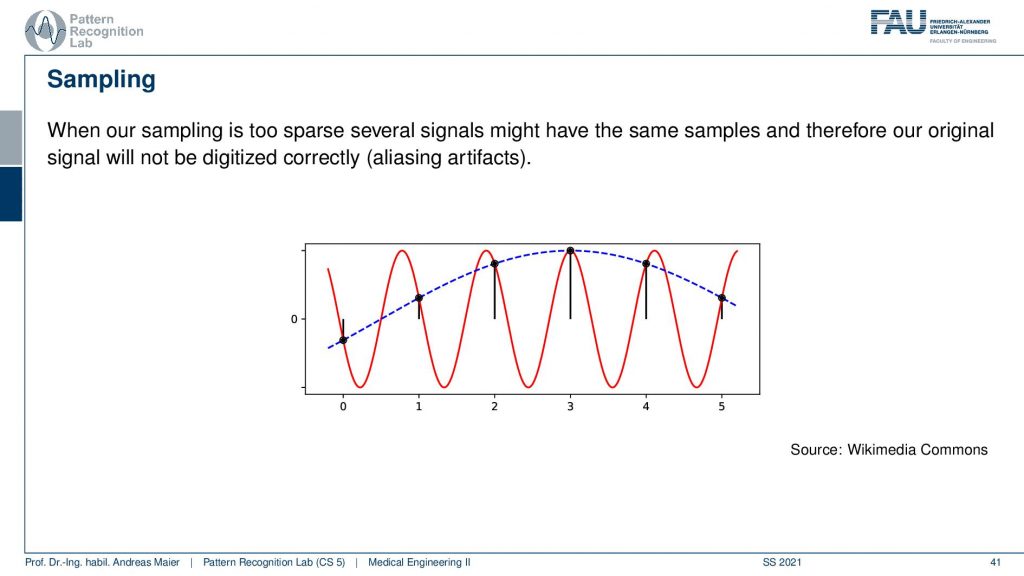
This is what I want to show you guys here in this plot. So here I have an input signal and this is the red curve. Now I decide to sample at the black dots and you see that I chose them at some arbitrary spacing. What you can see in this example is I always have the same distance between the black dots. So I get some values and the values are created exactly where the sampling frequency then hits again our red curve. So I produce those black dots. Now I have the black dots and I want to restore the original signal. If you look very closely you see that these black dots can be explained by a different sine wave. They actually can be explained by a sine wave of a much lower frequency and this effect is called aliasing. As soon as you do a wrong sampling what will happen is aliasing. So you’re no longer able to reconstruct the original signal and it’s not just that there are faint mistakes or something if you do the sampling wrong you get completely different signals. So they look entirely different because you didn’t obey the sampling frequency. This is also an effect that emerges if your visual system is being oversampled then there are certain effects that you can’t explain. I think the most frequent analogy that we find in the human visual system is the sampling of a spinning wheel. If a wheel rotates too quickly you can see that the actual wheel seems to be turning backward. This is because your visual system is exposed to a frequency that is higher than something that it can actually explain. It will then reconstruct in your brain a signal that doesn’t make sense. The fast-spinning wheel then looks like it’s turning backward. This is because it is rotating at a frequency that your perception is not able to comprehend and then you’re reconstructing something that doesn’t make sense.

So this is crucial and it’s very important. There is the Nyquist-Shannon sampling theorem which tells us how to pick the sampling frequency correctly.

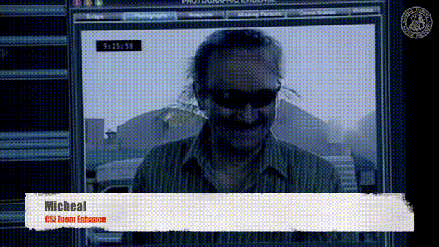
It states if a function x(t) contains no frequencies higher than B Hz it is completely determined by giving its ordinance at a series of points spaced 1/(2B) seconds apart. So if we sample at a frequency that is twice as high as the highest frequency in the signal, we are able to restore the entire signal without any loss. So this means that our sampling distance ∆x must be equal to or smaller than half of the size of the shortest wavelength. So the shortest wavelength divided by 2 gives you the step size on your x-axis. So this is the sampling step size ∆t or if you convert it to frequency domain it would be the sampling frequency. This is quite important and this has several implications. In particular, if you have a digital signal that has been sampled at a certain frequency then there is no way that you can reconstruct frequencies from this that are higher than half of the sampling frequency. They will simply be lost. They will be mapped to lower frequencies. So if you have a digital signal then there is no way how to figure out what the highest frequency is in this digital signal unless you know that it was correctly sampled. It’s very very important and if you already have digital data and it wasn’t digitized properly you don’t bring this back but you will get those aliasing artifacts. Well, there’s one way how you can bring it back. That is the process of so-called super-resolution and this is something that is an advanced class. We won’t talk about super-resolution here in this course but we have other image processing courses where we talk about image super-resolution. Here the idea is that you know the system’s relations to each other and you have multiple observations of the same original system. For example, you know that the sampling pattern was shifted to each other and then you’re able to reconstruct the super-resolved signal from the information that is contained in the aliasing artifacts. Of course, you get a big problem if you used a filter before the digitization that gets rid of higher frequencies. Because that would mean that there is no aliasing or effects. So be careful with super-resolution but we don’t discuss it here. By the way, if you see things like CSI, where they reconstruct suddenly super sharp images from very old video footage, it’s all nonsense. It doesn’t work and well if it would work then you probably would have to embed prior knowledge and that then just means that you’re reconstructing something that comes from a different source but for sure not from this video footage.

Anyway, we have a couple of implications that we’ve seen by this sampling frequency. Now I want to show you a couple of sampling frequencies that are quite common in several applications.

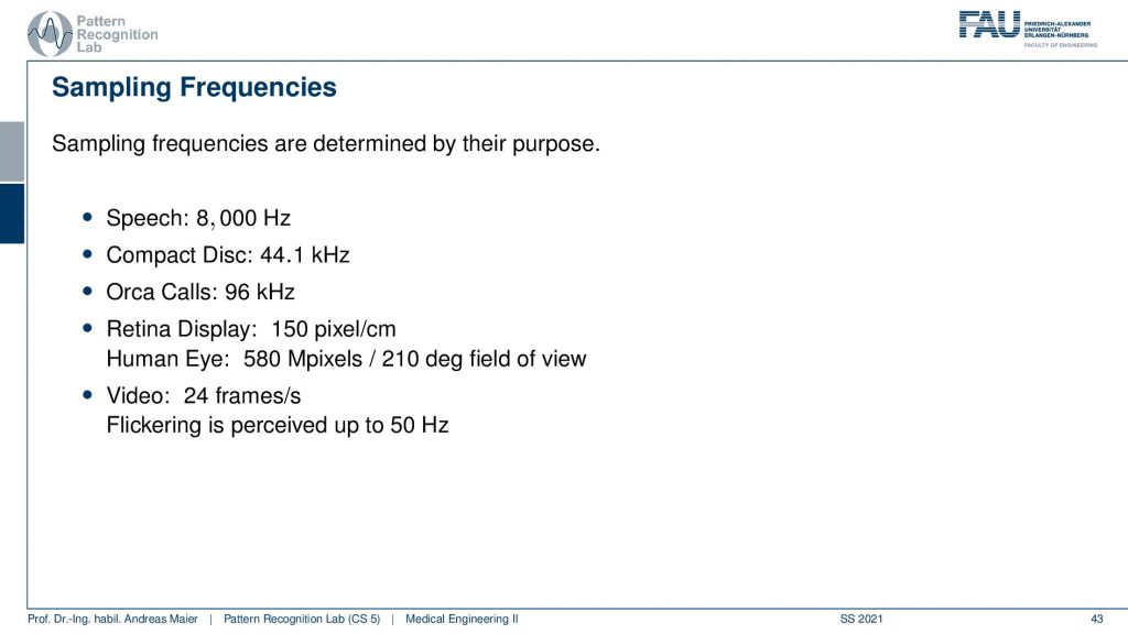
So this is not only the medical domain but some domains where you know signals and digitization probably. So speech for example has a maximum frequency of 8,000 Hz. It is the maximum frequency that is contained in speech which means that if you are sampling at 16 kHz you can reconstruct speech entirely. So your articulators your mouth and vocal folds and so on they are not able to produce frequencies that are higher than 8,000 Hz. Sometimes you have also telephone channels that have a reduced frequency so they sample only with 8 kHz. So, for example, some mobile phones used to have that in older standards. In these channels, you will have trouble differentiating certain sounds. So for example you’re not able to differentiate f and s. So if you look at my lips you will very clearly see the difference between f and s. So these are both fricatives and the fricatives have essentially the highest frequencies that are contained in human speech. So these are essentially the noises that are generated by the ssshh(s) and fffhh(f). They cannot be differentiated over some telephone channels. So be careful when you use those channels and this is also the reason why when people are spelling certain characters they introduce the natto alphabet. Because sometimes the information cannot be encoded over that channel and then you find surrogates in order to make sure that the correct information was transmitted. If you think about compactness so audio then a very frequent frequency limit for sampling is 44.1 kHz. So this was the sampling frequency of the compact disc. You may not remember this is a cd. Maybe you’ve seen that with your grandparents probably don’t have stuff like this at home. Because everybody is using streaming and mp3 players anymore. But the cd, the compact disc had a frequency limit of 44.1 kHz. By the way, this is very evil punk music so you probably want to don’t want to listen to this anyway. This is because human perception human hearing has a frequency limitation of 20 kHz. So you can’t hear things that are above 20 kHz. If you have very good hearing you may be able to hear frequencies above but it never goes beyond 22 kilohertz. So even the best perception stops at 22 kHz which means that if you sample at 44.1 kHz you will not be able to distinguish the digital signal from the original analog signal and it’s a perfect reconstruction. So this brings us to the 44.1 kHz in the compact disc. If you have other species like Orcas, Whales; when they sing the orca calls you have to choose higher sampling frequencies. So there you need to pick at least 96 kHz in order to be able to really get the full information. So if you listen to orca calls sometimes in you know television broadcasts they have been resampled. So they have been compressed in order to be audible for the human ear. So this is if you want to really hear the entire call you need frequency compression in order to make it audible for a human being. Also, the vision system has frequency limits and one is for example the retina display. If you heard about that this has 150 pixels per centimeter and this is so small that you’re not able to see the individual pixels anymore. So this is why they called it the retina display because it has essentially a resolution that is on par with the human retina with the resolution of your eye. If you would want to have the highest resolution on the retina for the entire field of view then you would need a camera with 580 megapixels. So a 580-megapixel camera over a field of view of 210 degrees would be able to sample the entire visual system of the human. Note that this is at full resolution but your eye is not built like a camera. So you don’t have a uniform resolution over the retina. So there are areas like the phobia where you really have the high resolution. But in the outskirts, you don’t have this high resolution anymore. This means that the 580 megapixels would only be required in order to sample everything as full resolution. Your eye is using many many tricks in order to give you the impression that you have this resolution over the entire field of view. Because it memorizes where you looked at and saves the high-resolution information and then places this back to your brain. So your eye is definitely not working as a camera system and it doesn’t have a uniform resolution which is of course also one of the reasons why there are so many optical illusions that suddenly you perceive something that isn’t there and so on this is because of the anatomy and the functioning of the eye. Also for a video you typically have 24 frames per second that are perceived as a continuous video by humans. But again your eye is not a camera system you can still see flickering up to a frequency of 50 Hz. So if you want to have a completely flickering-free impression you need a 100 Hz device in order to be able to get rid of any flickering effect. So this is why sometimes people like to buy 100 Hz television just to make sure that there is no flickering. I think with the LCD and OLED systems this effect is much less. But of course with the cathode ray tubes then you really had these half images per second and the flickering was much more of a problem. This is why people like to buy 100 Hz systems. If you talk to a professional gamer they will tell you they see the difference with 240 frames per second. So they need more frames per second just to be sure that they can be very accurate in playing their games. But according to research and what we know in published studies, 50 Hz should actually be enough. But you know if you’re a hardcore gamer and if you can beat everybody else maybe they have a super good perception that helps them to be on top of all the world ranking lists. So maybe they have a much better visual system than other humans.

Okay, so I think this is a key learning that you have here that digitization is driven by the purpose. Whenever you digitize something you need to know the purpose. This also drives us when we’re building medical imaging systems. We want to have a diagnostic purpose. So when we do medical images it’s not like with cameras or with you know human-computer interfaces where the human perception is the factor. But in medical imaging, the diagnosis is the relevant factor. So here all sampling and system design is done with respect to performing an optimal diagnosis. This is also why we use these many different systems and many different mechanisms. So here we have another purpose but generally, digitization is always driven by purpose. If the purpose changes you want to digitize it in a different way. 

If you have further questions send me a note, leave comments and get in contact with the online forums. It’s no problem we try to keep up with that as quickly as possible. Of course, I also have some further readings for you in particular in our textbook the chapter on systems theory by Peter Fischer.

It’s really well written it contains a lot more of the math. So there’s a couple of geek boxes that you can actually read this chapter twice once with a few math and then geek boxes with a lot of math. Maybe this is still a bit early, maybe you want to go back to the chapter in one or two semesters. There you can then really get all of the additional information all the additional math that we’re providing here. So it’s not just that this textbook should be a good companion for this class but it should also be a good reference when you’re in the field and you want to remember some things about systems theory or other modalities. Then you can go back to our book and review that specific chapter. It’s completely open access so you can download it for free and of course, it will also be downloadable for free in the future. So, of course, there’s also other very good reading and in particular the Einführung in die Systemtheorie. So this is a reference in german. If you do speak german then this is also a very good read and I definitely recommend having a look at that.

Okay, so this already ends our series of videos on systems theory. So you realize that this was a bit math-y. It will still stay a bit math-y for the next couple of videos. Because in the next videos we will look into the image processing part. So that we specifically now look at 2d images and how 2d images are processed. Again we will see the concepts of Fourier transforms, impulse responses, and convolution. These concepts will come up again. We will also discuss a couple of simple algorithms that can help you with improving image characteristics. So I hope you like this little video and I’m very much looking forward to seeing you in the next one. Bye-bye!!

If you liked this post, you can find more essays here, more educational material on Machine Learning here, or have a look at our Deep Learning Lecture. I would also appreciate a follow on YouTube, Twitter, Facebook, or LinkedIn in case you want to be informed about more essays, videos, and research in the future. This article is released under the Creative Commons 4.0 Attribution License and can be reprinted and modified if referenced. If you are interested in generating transcripts from video lectures try AutoBlog

References   

1. P. Fischer, et al., “System Theory”, in Medical imaging systems: an introductory guide, edited by A. Maier, et al. (Springer International Publishing, Cham, 2018), pp. 13–36, 10.1007/978-3-319-96520-8_2
2. B. Girod, et al., Einführung in die Systemtheorie: Signale und Systeme in der Elektrotechnik und Informationstechnik (German Edition), (Vieweg+Teubner Verlag, 2007)

Video References

• Javier Mota – Why do car wheels spin backwards on video? https://youtu.be/B8EMI3_0TO0
  
• Michael – CSI Zoom Enhance https://youtu.be/I_8ZH1Ggjk0

Category: Lecture Notes in Medical Engineering