
These are the lecture notes for FAU’s YouTube Lecture “Medical Engineering“. This is a full transcript of the lecture video & matching slides. We hope, you enjoy this as much as the videos. Of course, this transcript was created with deep learning techniques largely automatically and only minor manual modifications were performed. Try it yourself! If you spot mistakes, please let us know!
Welcome back to Medical Engineering and today we want to continue our little excursion through the theory. But you’ll see that we’ll get much more applied in the next couple of videos. Because in the next two videos we want to talk about actual 2-D signal processing and the first thing that we want to look at is an introduction to 2-D image processing. We’ll start with simple operations and expand them to linear systems theory and filters. Then in a second step, we will look into non-linear systems. So I hope you enjoy the 2-D image processing with me.

So here we will discuss the topic of image processing. So let’s have a look at the basics of image processing.
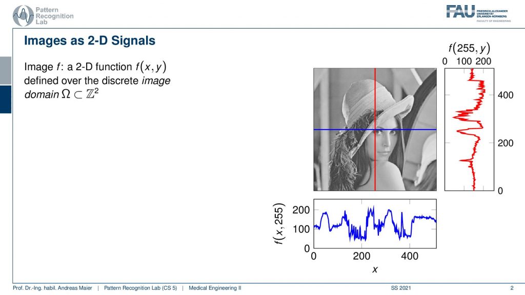
Now an image is essentially a 2-D function. You can think of the image as a function that essentially is on a grid space where you could say essentially every column and every row is a function or a signal as we’ve discussed earlier. Now we have to expand the space and be able to work with these 2-D signals. Here on the right-hand side, you see a visualization and you can see here that we have the red function which is essentially one column. This is a sequence of values that you can see here plotted. We also have the blue function which is essentially one row and it’s again a sequence of values. Together these gray values here in this example form a 2-D image. Now you see the lady here that is actually Lena and this is one of the first images that was used for image processing. It actually originates from a magazine that was published in November 1972. So at that time, there were not so many scanners and digital images available. It happened that one of those images was scanned. So they took a subsection of one of the largest images that they could find in the magazine, they scanned it, and actually, this image became kind of iconic and has been used in image processing over and over again. So Lena became extremely popular and she has also been invited although she didn’t know about her fans in the image processing community. So she has been invited actually to a couple of conferences and she is still being welcomed warm-heartedly at various conferences. Today people still use this image in order to test their algorithms. Well actually there are many other image sets that people experiment with now, but sometimes for nostalgic reasons this image is still being used. Note that only this subsection that we are showing here is being used and the full image is not being commonly used in the image processing community. So just that you don’t get the wrong impression. It was just one of the images that was lying around and that they had access to and they decided to use the subsection of the image. Well, what’s the digital image?
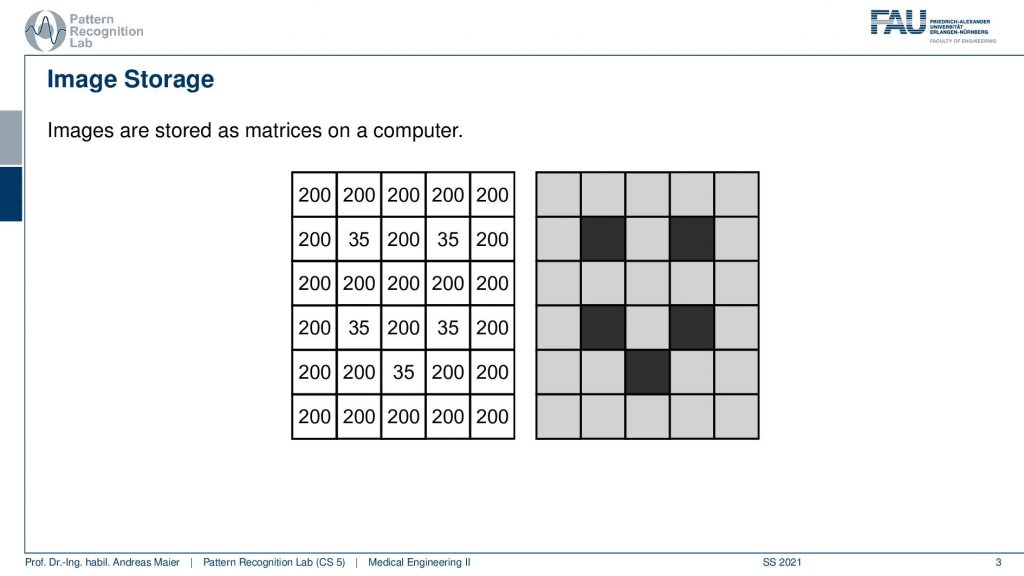
So let’s go back and think of our function space and what you can see here is a highly magnified image. So this is just showing a couple of black and gray dots. What you see here is that essentially every color every shade of gray is associated to a value. So the gray that you can see here it’s a light gray. So it’s associated to the value 200 and the dark color black is associated in this example to the color 35. So essentially every shade of gray is associated to a number and this number originated from a sampling process as we discussed in the last video. Obviously, these are the images that are used to introduce image processing.
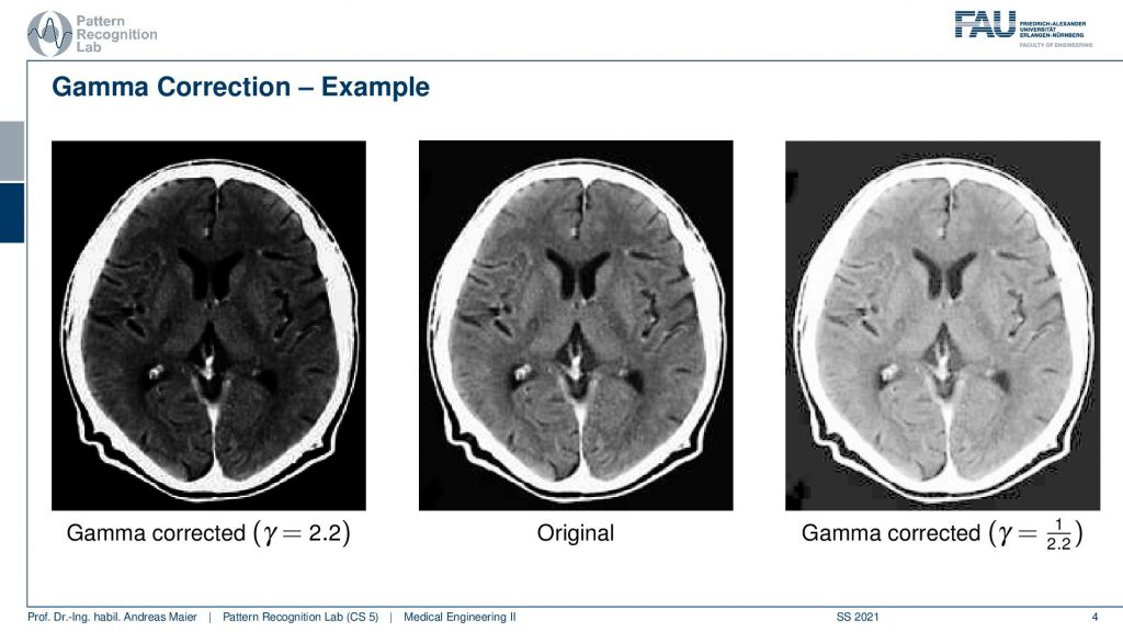
What we will work with much more frequently are of course medical images. One thing that is very peculiar about medical images is that they often have more gray values more shades of grey that you can actually show at the same time on your monitor and actually more than you can perceive. So the human visual system can approximately differentiate 256 different shades of gray. You cannot differentiate more or the average human being cannot differentiate more and if you display them you will see that they appear as a continuous color gradient or gray or gray value gradient on your screen. So in order to be able to visualize all of the information that is in the medical image, we have to use tricks. One trick that you could come up with is using different gamma values. You can see them here we can do a gamma correction which is a non-linear scaling of the gray values. If we would do so we would be able to focus more on the skull or on the brain and change the color values. This however is not so frequently used in medical imaging.

What is much more common is so-called window leveling. So here we have an example of a CT image and we know that Hounsfield units denoted as hu here are associated with different materials. On the left-hand side and the right-hand side, you see exactly the same image but displayed in a different window level. So minus a thousand Houndsfield units is air and plus a thousand Hounsfield units are bone or contrast agents. You see here that we can visualize all of the materials on the left-hand side ranging from air up to contrast agent that you can see in the heart and the bones. Then on the right-hand side image, waterish material such as water and soft tissues are around zero Hounsfield units. If we pick a threshold that is above zero HU, only the contrast agent and the bone will be visible. So what you see in this image are the contrast agent in the heart and the bones and you see that this is an interventional scan. So there is still some residual artifact that you see at the bottom of the scan. This was caused by truncation at the end of the volume. So also sometimes these scans have associated artifacts and you have to know about the problems that can arise in the scanning process in order not to misread the information here. So for sure, there is no ring-like bone structure at the bottom of the scan here. But this is artificially created by the reconstruction method. If you’re reading these images if you’re interpreting these images you have to know about this. Obviously, there is a wide range of variations that you can pick for windowing and thresholding and this is why I have a short video where we are playing with the window and threshold in different settings.
So what you see is that the image is actually composed of different gray values. Now what I’m showing here is called a histogram.
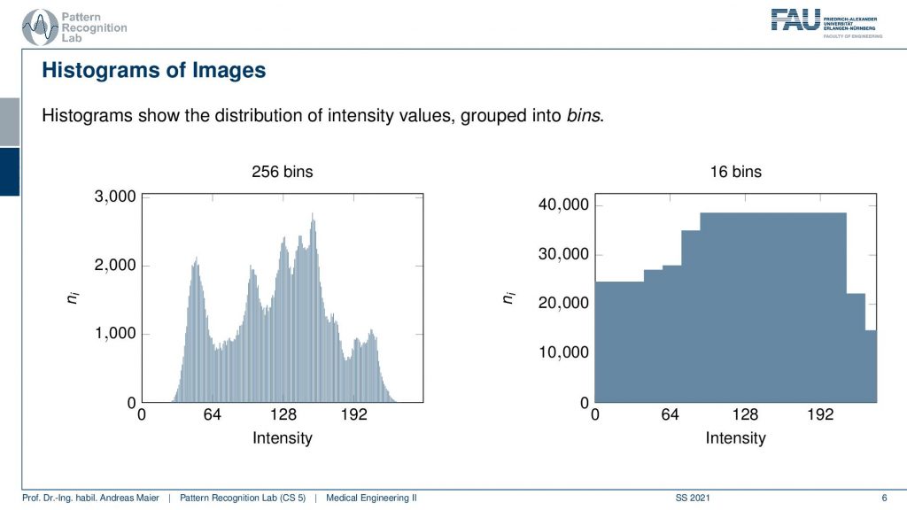
A histogram is essentially a kind of probability distribution because you count the frequency of the occurrence of every gray value. So on the left-hand side example, we have gray values from 0 to 255. So 256 different shades of gray and you can see on the y-axis how often that respective color or gray value appeared in the image. So the histogram doesn’t contain the spatial information anymore but it tells you which gray value occurs how frequently. Now if we change the window and level what we’re essentially doing is we’re adjusting the histogram. Here on the right-hand side, you can see a rescaling of the same histogram to only 16 bins. So here we have pooled neighboring gray values in order to reduce the number of gray values in that particular image. Obviously, this would have a large impact on the displayed image. You could immediately see that I adjusted the number of gray values. So this is something that we won’t do in the following. Now let’s go back to our example image.
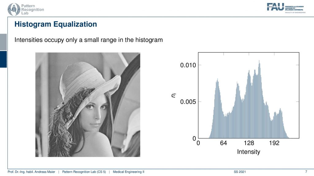
So here you see our famous Lena and if you look at the associated histogram here on the right-hand side you see that actually not all of the 256 gray values actually appear in the image. So you see that there is a short area with very low gray values and very high gray values where the frequency is zero. So they never appear in the image and you can see also that our Lena well the image impression is kind of okay. But she could use a little bit more contrast right? So this is where histogram equalization comes in.
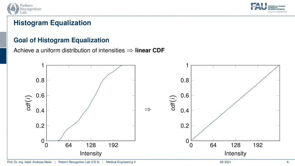
In histogram equalization, the idea is that we want to optimally use all of the associated gray values. What we’re doing here is we’re showing the cumulative density function which means that we’re essentially computing the integral over the histogram. So at every point in the cumulative density function, I am showing the addition of all the values from the zeroth bin to the current bin. So this can be computed essentially with a for loop where you then add up all of the previous values and write them into the respective bin. Now if I normalize this with the total number of pixels in the image you will see that we get values between 0 and 1. If you look at the left-hand side image you see the cumulative density function of our original image. You can also see that plateaus at the very low values and at the very high values where we don’t have any change in gray values anymore because these gray values simply do not occur in the image. Now the idea of histogram equalization is that you transform this cumulative density function on the left into the one on the right. So we want to linearize the entire cumulative density function which essentially means that we try to achieve a more or less uniform distribution of the grey values. There are algorithms to do so and in particular, they then introduce small gaps in the histogram such that all of the gray values are being used. So you could say this is very similar to what we are achieving when we apply the window leveling.
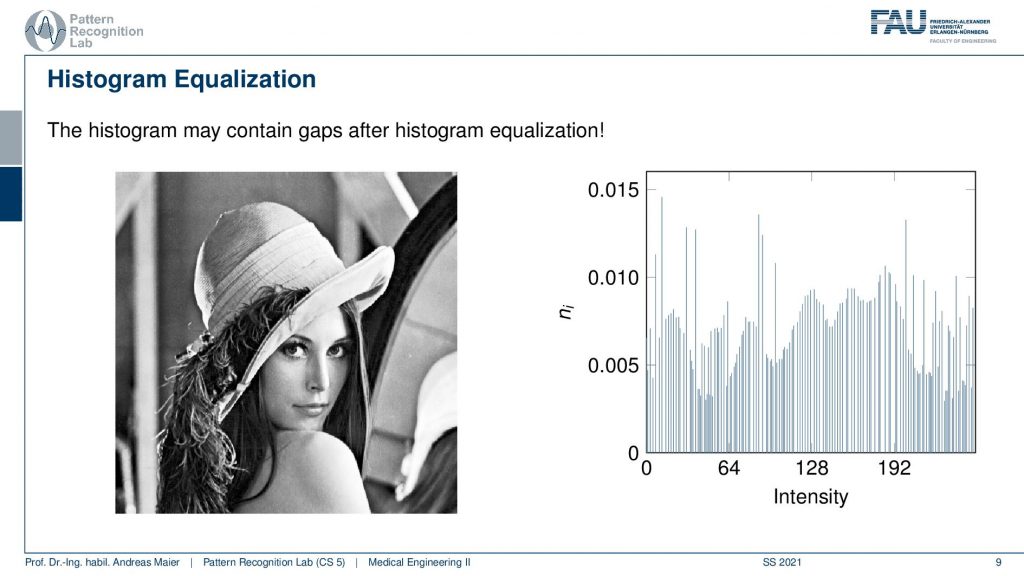
Now here you can see a histogram that has been equalized and now the contrast of the image has been improved. You can see that our lowest gray value is now really zero and the highest gray value is really 255. Let’s compare the two images.
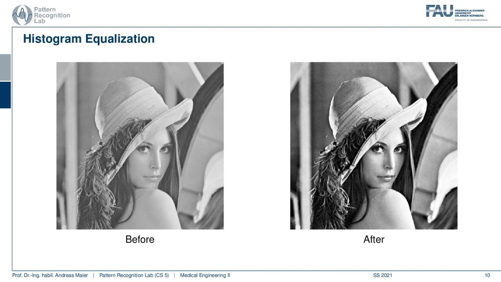
Here you can clearly see that the right-hand side image has much better contrast than the left-hand side image. Good! So these are the very basics of image processing. Now we want to go ahead and look at what we can achieve with linear systems theory.
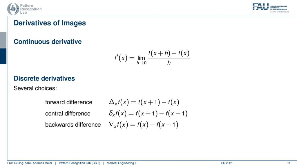
One thing that can be very nicely achieved is computing derivatives. Now a derivative of a function if you look at the definition: this is essentially the limit of the function plus a small value at the position x. Then you subtract the original value at position x from that and divide by the small value h. If you now have the limit of h towards zero you get the continuous derivative. Now the problem that we have is that we are in a discrete space. In a discrete space, we cannot assign values of h that are lower than one because they would be zero and then our whole computation would simply collapse to zero. So what we do is we then choose different variants of doing a single step size of 1 and then you come up with the solution shown here at the bottom. So you can for example take the value of 1 for h then you add 1 to the function f(x) and subtract f(x) from that. This would be the forward difference. There is the backward difference where you set h to minus 1 so you subtract 1 then the 2 flips and you have f(x) minus f(x-1). So the problem with those two approaches is that you’re essentially computing the derivative at the position x plus 0.5. So you’re kind of shifting the coordinate system and you wouldn’t be in the original coordinate system which is the reason why very frequently there are also central differences. The central difference then simply takes the pixel on the right-hand side and subtracts the pixel on the left-hand side of the current position of the image. This is interesting because it allows us to compute image derivatives. Now, why would we be interested in image derivatives?
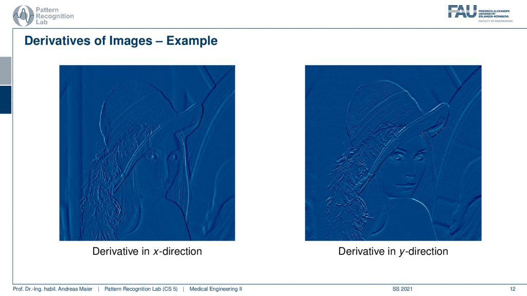
Well, let’s look at an example, and here you can see the derivatives in the x and y-direction. What you see very nicely here is that the edges pop up. So edges in our image are locations of very high gradients. So here you have either in x or y directions very high derivatives. So one idea for example to detect edges is to compute the derivative and x and y-direction. Then compute the magnitude of the two. Because you have a two-dimensional function. You will be introducing a gradient that is also two-dimensional because you compute the derivatives in x and y-direction. Then you take the norm for example the L2 norm of this gradient and this way you can determine the magnitude and detect edges. Interestingly, you can also compute the direction and then you could compute the angle of the edges which then allows you also to detect edges of a certain orientation. So this is a very very common application for linear systems and a good way of how we can actually compute edges in an image. This brings us back to image filtering and linear systems theory.
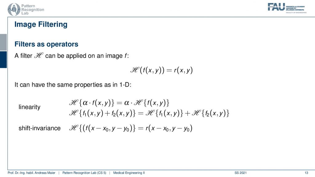
So you remember that a filter can be applied to an image. This filter has very similar properties as we already have discussed in the 1-D case. So the filters are linear and they are shift-invariant. So this is a linear shift-invariant system which means that it can be entirely described by convolution. Therefore we will need a 2-D convolution.
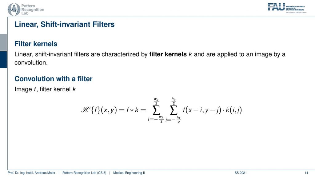
now you can see here that we have some function k which is filter kernel. The filter kernel now takes the role of the impulse response that we talked about earlier in our systems theory. So now we have certainly 2-D impulse responses and these can be written up in a discrete fashion. Then we end up with filtered kernels. For some functions, they can be described in a very compact way such as for the derivative we’ve seen at every point of the image we essentially have to take the left neighbor and the right neighbor subtract the two from each other and then we get exactly the derivative in that particular direction. So that’s interesting because we’ve just seen that computing a derivative can be performed by convolution. For a derivative, we can determine a kernel that is performing the derivative. So this means that computing derivatives are something that can be explained by a linear shift-invariant system. So that’s actually pretty useful and you’ll see that throughout your studies this will have many applications and it’s also very useful for example for solving partial differential equations. So you will see this will come up over and over again in your studies. Here we will now only stick to the discrete version and the nice thing with the discrete version is that we can write these up as these filter kernels.
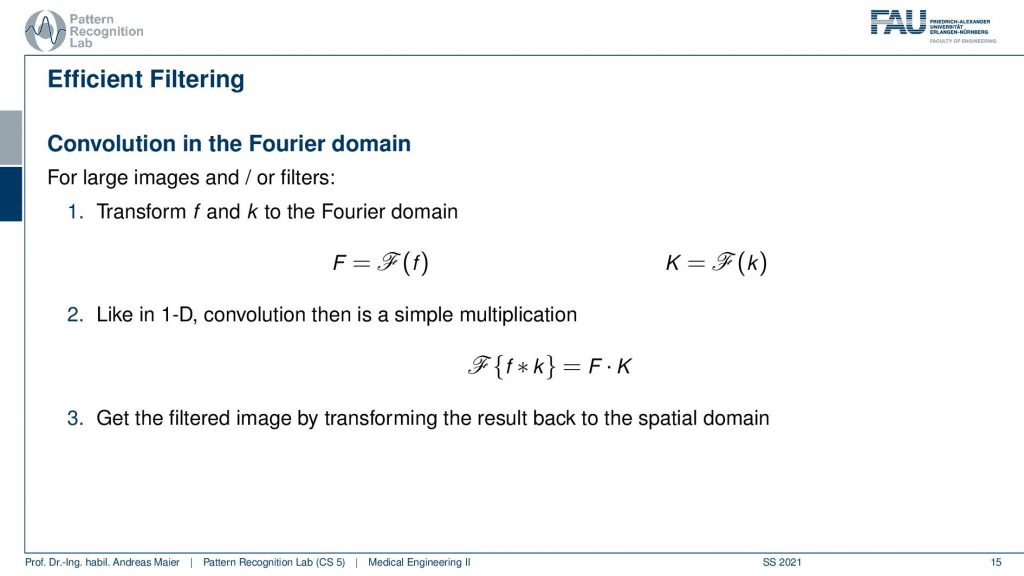
You will see that this then takes the form of very small masks for several filters such as the derivative filter. A side remark of course linear system theory applies and also the fundamental properties apply. This means that if you have a filter kernel and you convert it into a Fourier domain and you have the image and you convert it to a 2-D Fourier domain then you just have to multiply the two point-wise and convert back and you do exactly a convolution. Now for the simple filters that we have here in this set of slides, this would be rather excessive because typically the kernels are very small. They are like one by three or three by three or five by five. These are really compact kernels and there it doesn’t make sense to compute the complete Fourier transform. But sometimes you have kernels with a very large extent in the spatial domain and there it makes sense to make use of the Fourier properties. Also, you will see that the 2-D Fourier space is something that comes up in this class again and again. Now, what’s actually a 2-D Fourier space?
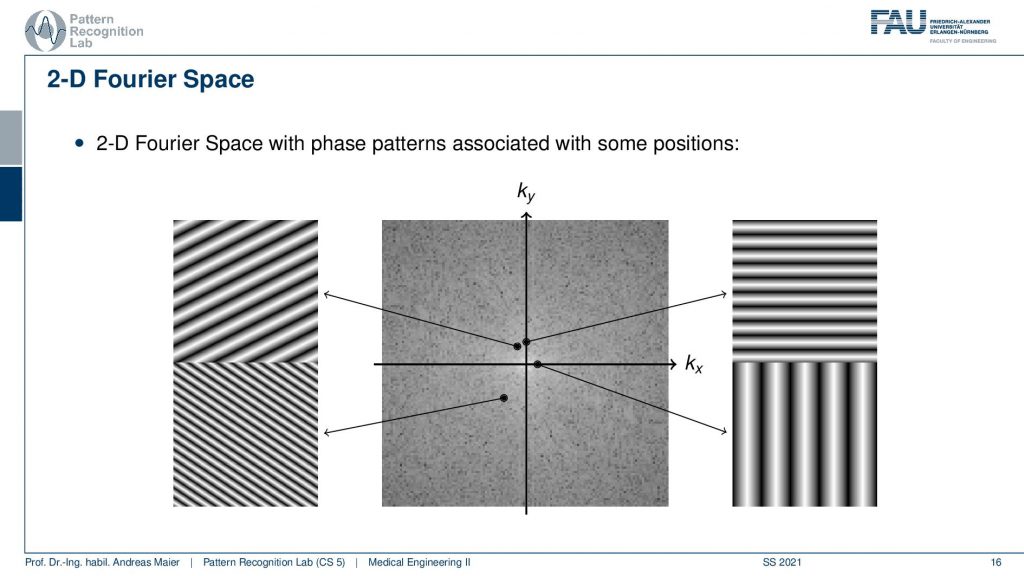
You remember that when we are computing the 1-D Fourier transform we essentially take a signal of a fixed frequency. Then we multiply it pointwise with the signal that we want to process, sum everything up and we get the coefficient for that particular frequency. Now in the 2-D case, this is slightly different. Because now our 2-D waves have to be described also in 2-D which means that it’s not just the frequency of the wave but they also have an orientation. So they’re essentially sine and cosine wavefronts that have a particular orientation and you can see that they have printed here the base functions on the set of slides. They vary in orientation and in frequency. So the frequency you can determine by looking essentially from one valley to the next valley. So that’s the wavelength and this is associated with one over the wavelength will give you the frequency. So what you see in this image now is that we can compute one point in the 2-D Fourier transform by taking one of the wavefronts that you see with different orientations multiplying the entire image pointwise with this waveform and summing everything up. This will then give you exactly one point into the Fourier space. So this is actually quite expensive to compute because we have to instantiate all those wavefronts. Then we have to multiply them pointwise with the image and add everything up and then you just got one point in the 2-D Fourier space. Also, see that the farther you go away from the center the shorter the wavelength gets and the higher the frequency, and the closer you get to the center the longer the wavelength and the lower the frequency. Also, note that depending on the orientation the direction that you’re at the orientation of the wavefront changes. Now if you look at this image then you can also see very easily that if you would be rotating the image then essentially you’re also rotating the 2-D Fourier space. So if you have a rotation in the spatial domain this will also be a rotation into the Fourier space. That’s quite interesting! So keep that in mind. If you want to go to Fourier space you have to compute those wavefronts multiply them point ways with each other and add them up. If you want to go back it’s the same as we discussed earlier. So you take the coefficient at that particular point in the 2-D Fourier transform you multiply this with the complete 2-D wavefront. Then you repeat that for all of the points in the 2-D Fourier space and add everything up. This way you get the original image again.
Let’s return to our example and now let’s discuss the filter kernel.
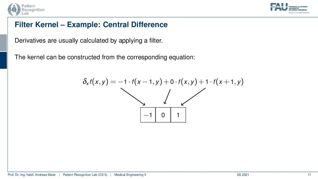
So the filter kernel here for the derivative filter of the central difference is simply this three-by-one matrix. So you simply have the derivative with respect to x written up here. So you take minus 1 times f(x-1,y) plus 0 times f(x,y) plus 1 times f(x+1,y). This is now the impulse response of the filter kernel that you have to convolve with in order to generate a derivative in the x-direction.
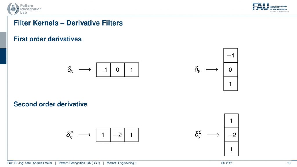
So for computing the derivative in y-direction you have to transpose the kernel. Then you get the solution here on the top right which will be able to compute the derivative in the x-direction. By the way, there are also second-order derivatives and the second-order derivatives can be determined also in a discrete fashion. Here this is simply the convolution of the kernel with itself. So if you convolve the x kernel with itself you get exactly the 1, -2, 1 and if you look at the shape of for example a Gaussian and its second-order derivative then you can see that you get these Mexican head types of functions. This is also represented here in the second-order derivative kernels. Also if you want to compute the y-direction then it’s simply the transpose of this kernel. There’s a couple of more kernels that we can come up with and here for example there is the mean filter.
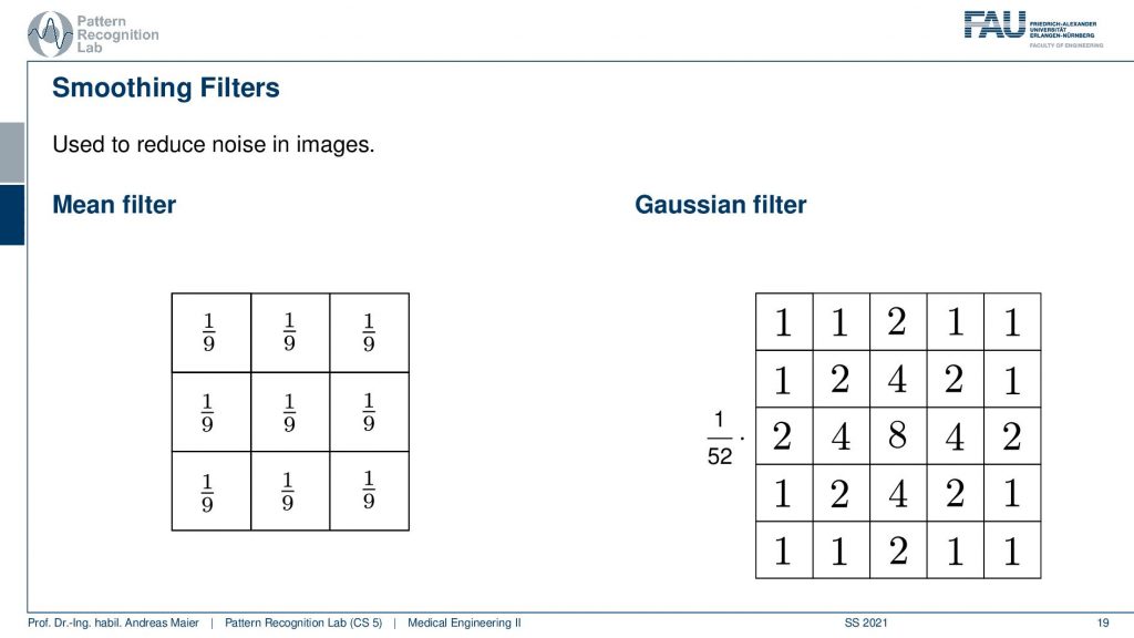
So here you have a neighborhood of three by three in total nine. So you take a kernel of an impulse response that is simply 1 over 9 at every position in that image. This is then also called the box filter. There are also discrete approximations of the Gaussian. One example here is shown on the right-hand side. So this is a 5X5 kernel and if you look at this and think about how the shape looks like you can see that this is a discrete approximation of a Gaussian bell in this discrete 5×5 neighborhood. Now if you take those filter kernels and apply them to the image you can observe the following.
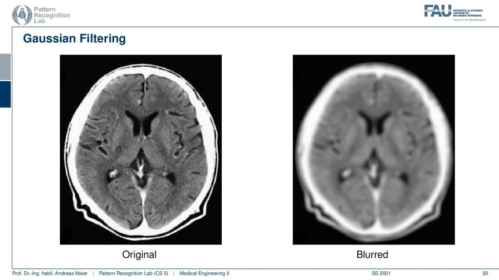
So both the mean and the gaussian are blur filters. So they reduce noise but also reduce the resolution of the image. So you can take the image on the left-hand side and produce an image like on the right-hand side here. There are actually many different kernels you can try. I also prepared a short video where we explore the use of a blur filter as well as a derivative filter using image j and I think this is something that you can very easily test with the software that we are also using in the exercises. So I would recommend actually playing around with eclipse and ImageJ when you’re writing these plugins. Also, give a short at the different functionalities of ImageJ you will find that this is really useful and many of the things that you find in photoshop or other image processing and software toolboxes can be rather easily be implemented on your own using filter kernels. Blurring, sharpening, and so on are essentially linear shifts and varying filter kernels and can be expressed by convolution.
I hope you enjoyed this little video here. I would be very delighted to see you again in the next video when we are discussing non-linear filters. So thank you very much for watching and bye-bye.
If you liked this post, you can find more essays here, more educational material on Machine Learning here, or have a look at our Deep Learning Lecture. I would also appreciate a follow on YouTube, Twitter, Facebook, or LinkedIn in case you want to be informed about more essays, videos, and research in the future. This article is released under the Creative Commons 4.0 Attribution License and can be reprinted and modified if referenced. If you are interested in generating transcripts from video lectures try AutoBlog
References
- Maier, A., Steidl, S., Christlein, V., Hornegger, J. Medical Imaging Systems – An Introductory Guide, Springer, Cham, 2018, ISBN 978-3-319-96520-8, Open Access at Springer Link
Video References
- Tyler Moore – 2D Fourier Transform – Fundamentals https://youtu.be/LSbMB0QyrYk