These are the lecture notes for FAU’s YouTube Lecture “Medical Engineering“. This is a full transcript of the lecture video & matching slides. We hope, you enjoy this as much as the videos. Of course, this transcript was created with deep learning techniques largely automatically and only minor manual modifications were performed. Try it yourself! If you spot mistakes, please let us know!
Welcome back to Medical Engineering: medical imaging systems. So today we want to talk a little bit about a concept that is called convolution. Convolution is a very useful means of computing functions and we will see that it’s also a super useful tool if we want to describe systems that are acting on signals. So please stay tuned for a short introduction to convolution.

Today we want to discuss the concept of convolution and you’ll see that convolution is one of the basic operations that you can apply to functions. So it is essentially a kind of transformation that is as useful as addition or multiplication if you’re dealing in function space.
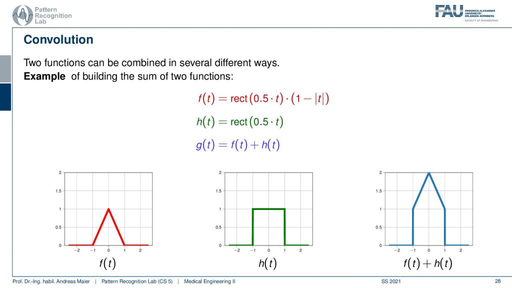
So we know that we can combine different functions with each other for example by multiplying or by adding them to each other. Here in this example, I have two functions the red one that is f(t) is essentially a triangular function. Then we have the green one which is h(t), a rectangular function and then we have the output g(t) which is some combination of the two functions. Here we use the addition and you see if I add a triangle to a rectangular function pointwise I just get the function here on the right-hand side. So this is the kind of introduction to convolution. We want to use a new concept of combining two functions. Now convolution is a different trick we also combine two functions but the output is quite different from what you know with multiplication and addition.
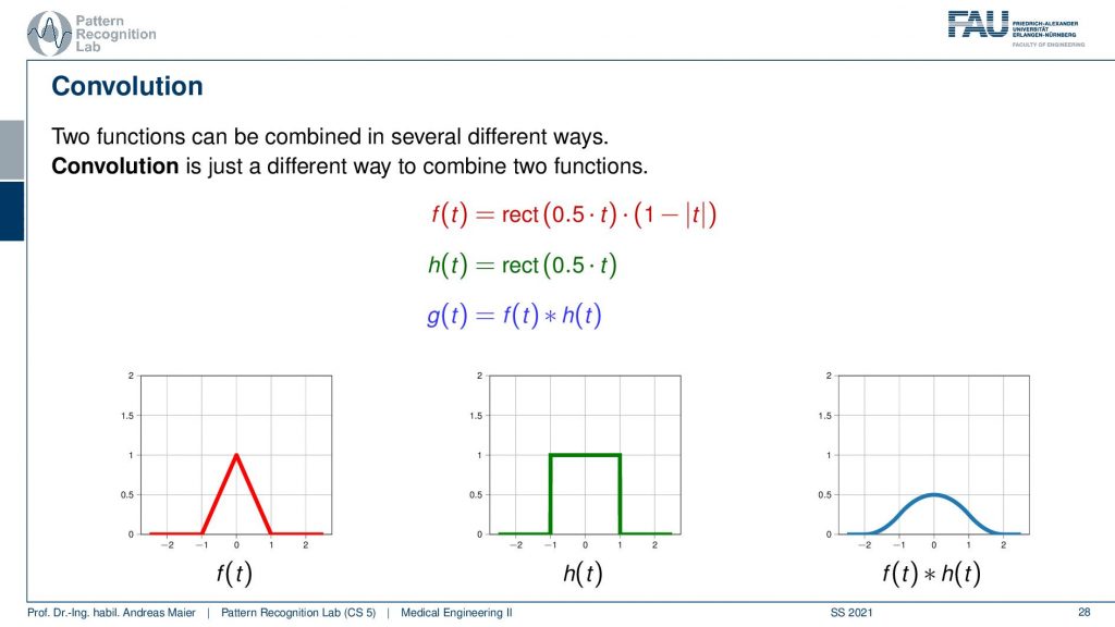
So if we convolve the two functions with each other then we get the one here on the right-hand side and this looks like this bell-shaped curve. So it’s very different from addition and multiplication, right? So let’s have a look at how this is actually computed.
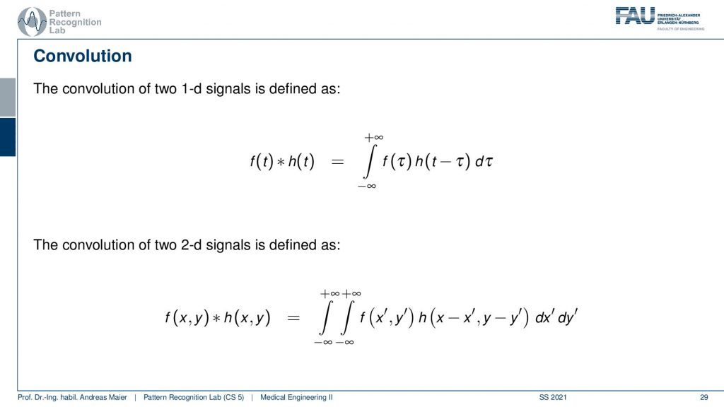
Now the convolution is integration from minus infinity to plus infinity and a point minus multiplication of the two and I shift one of the two functions by some variable tau. Then add the two up. So the convolution is essentially shifting two functions aside from each other and then we multiply the two and add them up. Obviously, this is also defined in 2d space and then we have a double integration and we have two variables that we are actually integrating on. The 2d version will become very important when we are actually talking about the imaging systems. So this will be the kind of topic that we are talking about in the video after the next video. So then we’ll talk about image processing. Now we’re only talking about 1d signals. So let’s look at 1d convolution.
This is our example we have the rectangular function and the triangular function. We shift the two against each other and then compute essentially the weighted integral over the two functions. So this is very easy here with the rectangular function. If I shift them like on the left-hand side then the multiplication of the two functions and the integral over this is obviously zero. So let’s shift it a little more and now we have the point where they essentially touch. So it’s a very slight touching. So still, zero, shift it a little more and now you see that they start overlapping. So I multiply them pointwise and compute the integral. Then I shift them a little more and you see now how the blue function on the right-hand side is slightly increasing. This is the output of the convolution. So if we shift a little more then you can see that the overlap increases the function value increases because the integration of the two functions increases. Then we can shift it a little more you see that the overlap goes down. So the function value goes down again. We shift more function value goes down again and even more and then we reach some point where they don’t overlap anymore. So this is a way how we can compute the convolution. We shift two functions against each other and then we multiply them and add them up and this results in the curve here on the right-hand side.
Let’s take a different pair of functions. This is such a strange concept. Let’s look at this again and now I’m taking two rectangular functions.
So I’m shifting again the green curve. Then they start touching so I start getting values. Now you see if I shift it’s a linear increase. So I essentially get this line but again the overlap then is reduced and it’s linearly decreasing again. So if I convolve two rectangular functions with each other I get a triangular function. That’s interesting and if I convolve a triangular function with a rectangular function I get this bell-shaped function. So that’s an interesting concept and this is how we can do convolution.
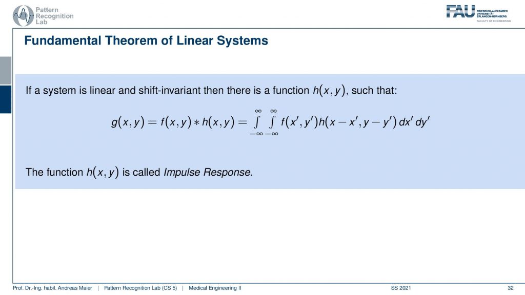
So a very important concept is the fundamental theorem of linear systems. If a system is linear and shift-invariant you remember two videos ago, if those two properties are fulfilled linear shift-invariant then there is a function h(x,y), so this is the 2d case here that describes the entire system. So we can express a linear shift-invariant system always using a convolution. Every linear shift-invariant system can be expressed by some function that is convolved with the original function. That’s cool! This function h(x,y) is called the impulse response. So the impulse response is able to describe the entire system. If you know the impulse response you’re done you know what the system does. That’s interesting! So linear shift-invariant systems perform convolutions and they perform convolutions with the impulse response.
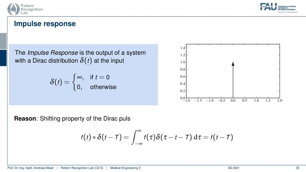
Now, what is that called impulse response? Well, it’s because the impulse is also called a Dirac distribution here. This impulse is the neutral element for convolution meaning if I convolve something with an impulse or Dirac distribution that is simply zero everywhere except at zero where it’s infinitely high. So this is really just a peak and then nothing else like you see here on the right-hand side. This is the neutral element for convolution. So if I convolve with this impulse I get exactly the original function and you see that here on the bottom it’s called the shifting property of the Dirac pulse. If I shift it with some variable t then I will get exactly f shifted by t when I convolve with this direct impulse. Why is this useful? Well, an impulse is just something that is very short right? So you need something very sudden and this allows you to describe the entire system. One thing that is for example true for audio processing is that you just need a click or snapping like this one. Then you can characterize for example the echo properties of an audio system. So if you look at the impulse response of my snapping here then you will be able to measure the acoustic properties of my microphone and actually the room I’m in and what the echo duration is in here. So echo is essentially a convolution. So if you’re on the mountainside and you’re yelling out into the mountains and then you hear the echo that is being reflected that is actually a convolution. The echo is simply returning what you said because it has a time delay and it just reproduces whatever you put in there. If you would be snapping then you would be able to characterize exactly the echo time of the mountain front that you’re using to generate this long-term echo.

So that’s interesting! This is the Dirac pulse and the response of the system. So you put in the pulse and then you get the response and this response is completely characterizing the entire system. In time processing it can be just this little peak. So you could have very short rectangular pulses that are below the resolution of the system that you’re actually processing with. If you’re doing image processing this impulse could be just a very sharp dot that you showed to the system. So this is also one way how you can measure the resolution of a camera system. You show just a tiny dot and this tiny dot is then able to describe the entire camera blur and so on. So these are also linear systems that can be described as very simple measurements actually. So we will see a bit more on that in the image processing videos.
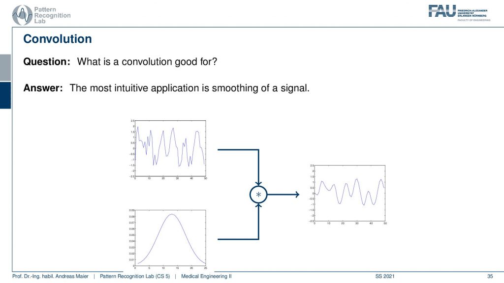
Okay so let’s have a look at some examples of what is convolution good for? Well, there is the most intuitive application that you can think of and it’s moving of a signal. So that’s a very typical case. So you have some input signal, it has noise. You remember the two frequencies that were overlaid and you were not able to figure out what it’s actually doing. Well you can apply for example this gaussian here and you convolve with it and then you get a very smooth signal. This way if you choose the filter appropriately then you’re able to denoise for example and restore the original information or the information that you are trying to decipher from the signal. This is one typical application.
There’s a little more to that because the convolution is also associated with the Fourier transform.
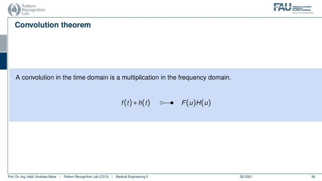
There is the so-called convolution theorem and it tells us that a convolution and time domain is a multiplication and frequency domain. This is also one of the reasons why the Fourier transform is so important for us. Because it allows us to describe systems, linear, shift-invariant systems entirely in the frequency domain. So I have this complex function that I need to shift the two and have a lot of computations in order to perform the convolution and time domain. But if I actually do that in the frequency domain it’s just a point-wise multiplication. If you go into some algorithm class later on you will see that there are also very fast versions of the Fourier transform that then can help us to compute convolutions very quickly. So the convolution is typically n to the power of two in terms of multiply-add operations and a Fourier transform can be performed in nlog(n). So this is a much more efficient algorithm and therefore in some instances, it really makes sense to work in the Fourier domain. So you do the Fast Fourier transform. You work through your space multiply the two signals and then transform back and you have exactly implemented the conclusion. So Fourier transform is very important in terms of theory and in order to understand the systems and their properties. It’s also very important for implementation and this is how you can save a lot of compute time if you use tricks like the fast Fourier transform.
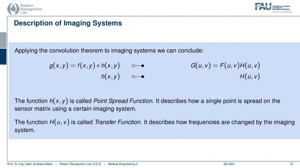
Now, this also applies of course to our imaging systems. If I have something like a convolution in the spatial domain that would be f convolved with h and I have the impulse response that is h(x,y) here on the left-hand side. Now I’m denoting this filled circle and the empty circle in order to transform it into the Fourier domain. Now you see that the equation g(x,y) is then transformed into a frequency domain variable where we then have u and v. So these are spatial frequencies of a 2d signal and there is still a pointwise multiplication of the two. So if I know H here on the right-hand side then I have the so-called transfer function. Of course, the transfer function and the point spread function here in this 2d case would be the impulse response if we had a time-domain signal. Then they two are just associated with each other with a 2d Fourier transform. We will talk about the 2d Fourier transform in a little more detail when we talk about image processing. But you can generally convert the two into each other either with 1d or 2d Fourier transforms. So the 2d impulse response is called the Point Spread Function because it describes the spread of a single point similar to the example that we just had with the echo. The echo train is just generated by this impulse here and if we look at the same function in Fourier space it is called the transfer function. This essentially describes how the different frequencies are affected by the imaging system here in this case.
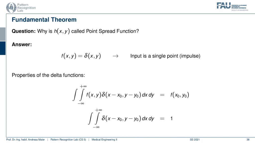
So why is this called the point spread function? Well if we had a Dirac pulse that is 2d it would be just a single point I already hinted at that. So this would be the point or impulse in 2d. Then again we have the properties of the Dirac function here that if we do a 2d convolution with the point spread function then we simply get the output at this particular location. So this is again the neutral element. So we are able to assemble the entire point spread function just using a single point and this determines our entire system.
Okay so today we learned about the convolution concept and we’ve seen that convolution is essentially a way of combining two functions and it is as essential as addition and multiplication if you work in systems theory. Also, we’ve seen that a system that is linear and shift-invariant can be completely described using convolution. This then brought us to the concept of the Dirac pulse and if I feed the Dirac pulse into a system, I measure the impulse response and the impulse response is completely characterizing the system. We’ve also seen that potential applications are smoothing or, in images then denoising of such convolutions. But we will see that convolutions are very very useful and they allow us to characterize really complex systems like camera systems, blur effects, and many different other properties. We will also see that they are really useful for edge detection when we talk about image processing in two videos from now. So also very important concepts and I hope you enjoyed this small excursion to introducing the concept of convolution. This concept will be heavily used. Convolutional will pop up everywhere in this class and we will reuse it very very frequently and you should definitely be familiar with this concept. Rest assured the concept will also be very important for the remainder of your studies. It will come again and again. Maybe you can follow the concept in this video already but you can also have a look at the textbook, where we have a little more examples. This is really a concept that will accompany you probably throughout the rest of your career. By the way, it’s also implemented in modern AI algorithms. There’s a whole family of so-called convolutional neural networks and even if you are more interested in AI and so on this concept will come over again and again. You will definitely need to understand this concept. Okay, I hope you enjoyed this little video and you found the examples useful. You can also give feedback. There is the opportunity to send feedback on our online learning platforms, but you can also leave comments in the comments functionality. I would be very glad if we could meet again in one of the next videos. Thank you very much for watching and bye-bye.
If you liked this post, you can find more essays here, more educational material on Machine Learning here, or have a look at our Deep Learning Lecture. I would also appreciate a follow on YouTube, Twitter, Facebook, or LinkedIn in case you want to be informed about more essays, videos, and research in the future. This article is released under the Creative Commons 4.0 Attribution License and can be reprinted and modified if referenced. If you are interested in generating transcripts from video lectures try AutoBlog
References
- Maier, A., Steidl, S., Christlein, V., Hornegger, J. Medical Imaging Systems – An Introductory Guide, Springer, Cham, 2018, ISBN 978-3-319-96520-8, Open Access at Springer Link
Video References
- Omar Bsoul – Convolution Animation https://youtu.be/SVCeaiy0VVY
- Brek Martin – Fourier Series Animation (Square Wave) https://youtu.be/k8FXF1KjzY0