Magnetic Resonance Imaging – Part 2

These are the lecture notes for FAU’s YouTube Lecture “Medical Engineering“. This is a full transcript of the lecture video & matching slides. We hope, you enjoy this as much as the videos. Of course, this transcript was created with deep learning techniques largely automatically and only minor manual modifications were performed. Try it yourself! If you spot mistakes, please let us know!

Welcome back to Medical Engineering. Today we want to continue talking about magnetic resonance imaging and in particular, we want to figure out how to use the magnetic resonance effect in order to actually calculate images. You will see that this is actually a very nice application of the Fourier Transform. So looking forward to exploring the actual image formation in magnetic resonance imaging with you guys. 

So this is today’s outline. We want to explore the principles of magnetic resonance imaging, slice selection, the spatial encoding, and then we want to explore the so-called k space. So k is the wavenumber and we want to explore the space of wave numbers. Then we see finally a comparison of slice selective versus volume selective 3d imaging. Then in the second part of this video, we want to talk about advanced applications like spectrally selective excitation and functional imaging. This is already something that I hinted at in the previous video. So let’s start talking about the principles of magnetic resonance imaging.

Now we really want to talk about imaging. So you see it here in red. So this is actually the part where we explain how to get the images. So far we excited all of the nuclei at the same time within the magnetic field. Now for imaging, we need spatial information. So we think about how to actually get these spatial properties out there. There are two concepts that are the slice selection and spatial encoding and both of them will be used in order to figure out where actually which information is coming from and both of them are based on the gradient coil system. 

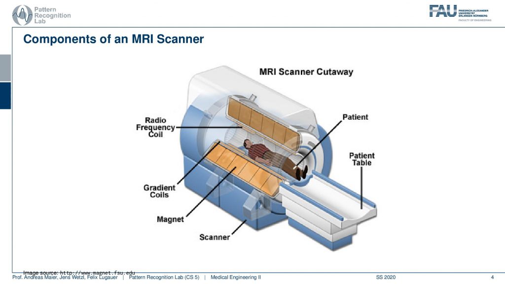
So let’s have a look at a cut view of such an MR scanner and here you can see what would happen if we would cut the scanner open. Well of course first of all we would get a huge quench. So all the liquid nitrogen would actually emerge but obviously, this is just a schematic. So what happens here is that you have the radio frequency coils. So they’re actually inside here in the coil system around the patient. Now you also see how deep the scanner is. We can fit the entire person in here. So this is our patient and we’ve already seen that there is a patient table that is used in order to move the patient inside here. Then there is the main magnet. So this is our main magnet which is the strong magnetic p0 field and we have the so-called gradient coils. The gradient coils are the ones that we use in order to steer the direction of the local gradient field. So why do we need these gradient coils? We’ve seen that we have the rf coils so we need them to excite and to readout. But now what are these gradients for?

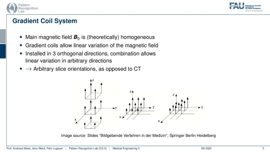
So the gradient coil system is a kind of system that allows us to modify the strength of the magnetic field locally. There are in principle free coils. So there is the so-called z coil that allows us to increase and decrease the magnitude of the field in that direction. Then there is the so-called x gradient field. So this changes then a stronger and weaker kind of magnetic field in the x-direction and we have the y coil. So the y coil then changes the strength of the magnitude in the y-direction and with these three coils, we can then essentially superimpose them over each other. This allows us to get an arbitrary type of change in the local B0 and this can help us to change the Larmor frequency at every spatial position inside of the scanner. 

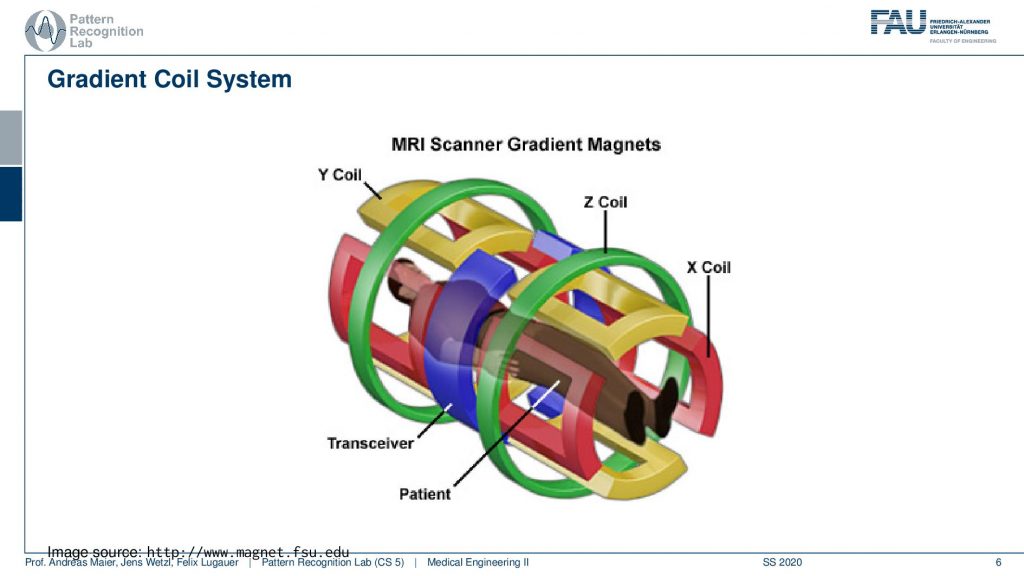
So if this is then implemented you can see here that we have now in a different color of course than on the previous light. So this is our x coil and these are essentially coils and they can introduce an additional magnetic field in this direction. The z coil would introduce it in this direction here and the y coil would introduce it in this direction here. So you see with our different coils. I actually should use this color here. So let’s use this color here. So this is our y coil. So we’re able to apply additional magnetic fields in all spatial directions. This is the gradient system by superposition of them we can essentially guarantee additional magnetization in any orientation. This is also the key component why we can apply these gradients in all directions and there will acquire images in all possible orientations. 

So let’s go ahead and talk about the so-called slice selection. 

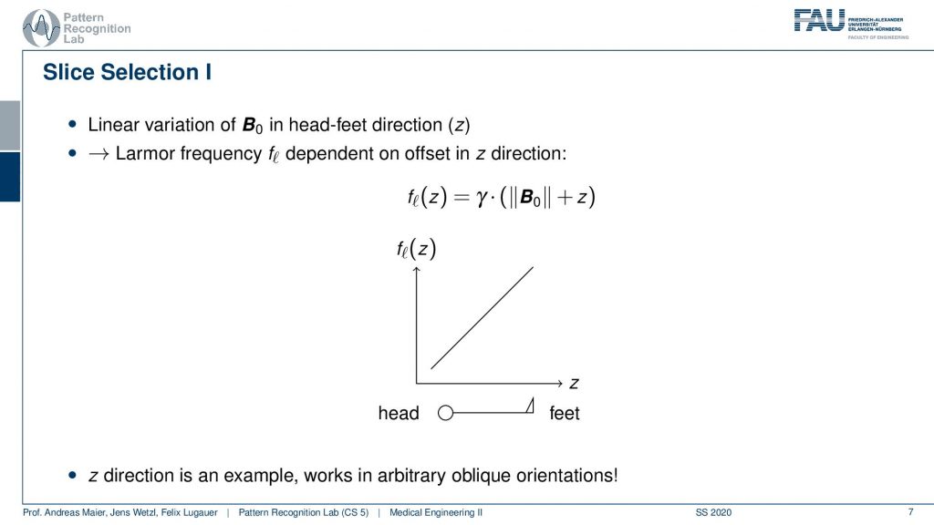
Now slice selection is the concept that allows us to select only a specific slice within the body. The idea is that we want to use the gradient in order to apply some additional magnetization z and this allows us to adjust the Larmor frequency of the respective voxel. So if you do that in z-direction then the additional set coil would increase the frequency towards the feet and decrease the frequency towards the head. Now because we excite only with a specific frequency and we can pre-compute that we can see that this would then align with a specific position in the body. So the gradient can be used to select only a specific slice within the body. and of course, with the superposition of the different gradient fields, we will be able to actually get any kind of orientation here. 

So how would we do it? Well, we would pre-compute at what frequency we actually have to excite. Then we apply a specific gradient and of course, we do that with the right steepness. We know that maybe we are exciting a little more because there’s some co-excitation of neighboring frequencies but we can then map this very nicely to a specific area within the body. So you see this way I can essentially determine by the steepness of this gradient. I can determine how thin the slice will be and if I take a broader direction then I will get very thick slices. With this idea we can then essentially determine which slice inside the body will be excited and therefore all the signals that we are measuring can only emerge from that particular slice. So you see here I have the neighboring directions that are being excited and this means that with our particular gradient we will only select voxels that are actually lying in this region of the body. So this way we can get an arbitrary slice excitation. 

Now we have to go ahead and somehow figure out where the signal is coming from within the slice and this is called spatial encoding. We will use some additional ideas that we can actually use again the gradient coils in order to introduce something which is called a phase shift. 

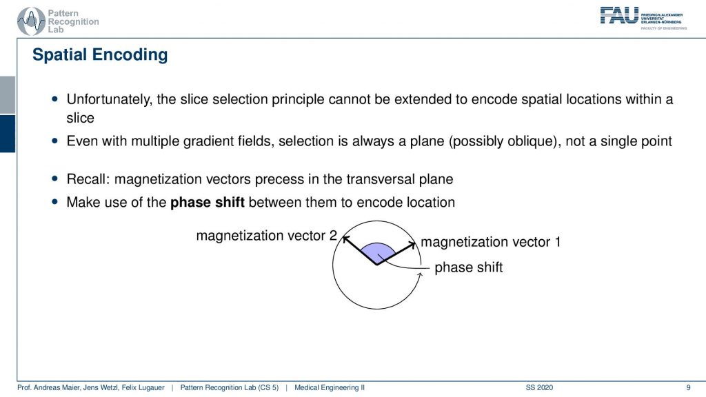
So how does this work? Well typically if we excite uniformly then all of our hydrogen nuclei will spin in exactly the same phase. So we excite them uniformly and then all of them will essentially rotate in synchrony. So we cannot use the slice and coding principle again but we can use a trick. We use again the gradient coil and then we again introduce a shift in the Larmor frequency. So what we can do is we can essentially change the local magnetic field after the excitation after excitation all of them rotate in synchrony and then we want to change the magnetic field locally such that some of the rotations are out of synchrony and this is then called the phase shift. So this kind of angle between the rotations is the kind of means that we want to use in order to differentiate different spatial positions.

So how this can be done? 

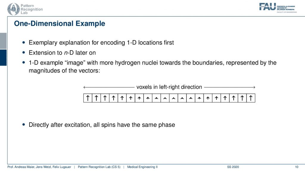
Well, let’s start with a one-dimensional example. Now we encode let’s just stick with the 1d example and we excite everything and then depending on the magnetization of the number of hydrogen nuclei within the voxel, we will get a different net magnetization. You see here we have many and here we have fewer and here we have many of them again. But they all are oriented in the same direction because we excited them in the same phase with exactly the same kind of rf pulse. So directly after the excitation all of the spins have the same phase. They all point in the same direction. 

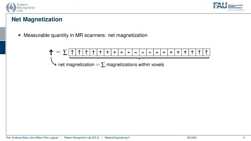
Now if I were to measure what I would measure from this set of voxels is essentially a sum. I get the superposition over the actually in the entire 2-D slice. But let’s stick with the 1d example first. My measurement is not able to resolve spatially. So I get the sum over all these net magnetizations and distance because they all point in the same direction. This gives us a net magnetization that now points towards the top. 

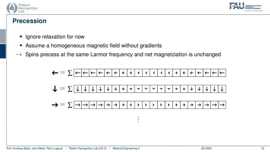
Now if this is done at a later point in time that’s not a big problem because they all rotate in synchrony. So if I measure a little later I might be measuring this here but the magnitude is exactly the same. It might be a different orientation but the sum will cause the magnitude to be exactly the same and because everything is rotating in synchrony I always get the same signal. So there’s not a big problem and they all process at the same Larmor frequency. So we always get exactly the same magnitude but a different orientation and all of them are of course oriented in the same direction because everything has been excited at the same time with the same frequency. 

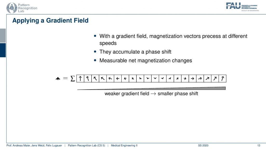
Now we can use a trick. We apply a gradient field and we apply the gradient field shortly after the excitation. This then causes that right after the excitation we have a different gradient field. So they are already excited. So we know only the spins within the slice are actually already spinning. Then we apply this additional weaker gradient field. You see if I apply this weaker gradient field I’m changing the local Larmor frequency and by changing the Larmor frequency they will start spinning at different speeds, right? Because the Larmor frequency is different. Then they slightly go out of phase. So if I now observe at the same point in time but I apply it in between the weaker gradient field and the higher gradient field at this point you see that they will be in a different phase, they will be rotated towards a different angle. So I apply this gradient field then I turn it off and then I measure. Now after turning this off everything will continue spinning synchronously. So I would again be able to measure the same magnetization in different directions because I kind of turned it off. So this net magnetization here will not change anymore. But now because we orient the arrows in different directions the sum will now no longer sum up to this large magnetization as we had previously. But it will be reduced. Now I can play with this kind of gradient and see how I can modulate the net magnetization of my vector. 

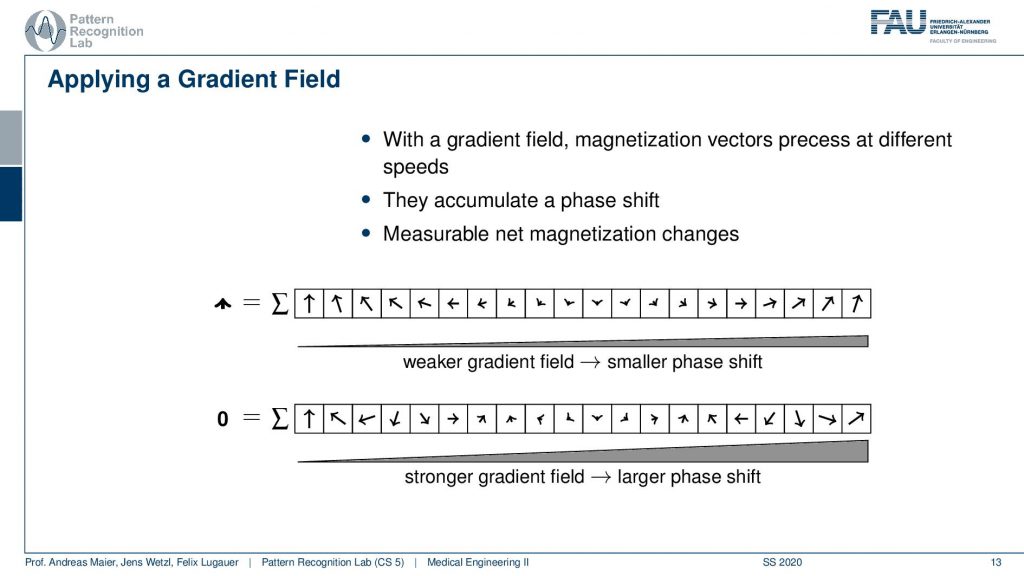
So this then could be employed with different kinds of magnetic fields. So let’s say I take a gradient that is stronger. So I have a stronger magnification or amplification here towards this side. Then you see in every time step we have a slightly higher degree of rotation. So we have a higher phase shift in every step here towards the stronger gradient. So we tilt a little more and then we measure again and suddenly our magnetization is zero. So if I have this kind of weak gradient field I have a slight reduction and I have this strong gradient field then I have a stronger reduction. Now you can see that the arrows here kind of form a pattern right. 

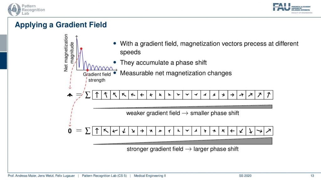
So you could argue now that if I did these two measurements then I essentially could plot the gradient field strength here to the right-hand side and the magnetization here to the top. Obviously, without any additional gradient field, I get the highest magnetization simply because everything is in synchrony and I have no effects of the neighboring voxel that they disturb each other. Now if I  start applying a weak gradient field I start reducing the signal and you can see then over increasing the field strength I get this kind of lobes. So I’m jumping up and down with the field trend and I generally have a reduction here in the general magnetization. But I can do this with repeated measurements and I get this different kind of resonance effect because I caused a different phase shift. 

Now, why would I want to do that? Well, you kind of can think of this phase measurement as measuring parts that are kind of in the same kind of orientation or you could even put it into a kind of interpretation where you have a certain kind of influence. 

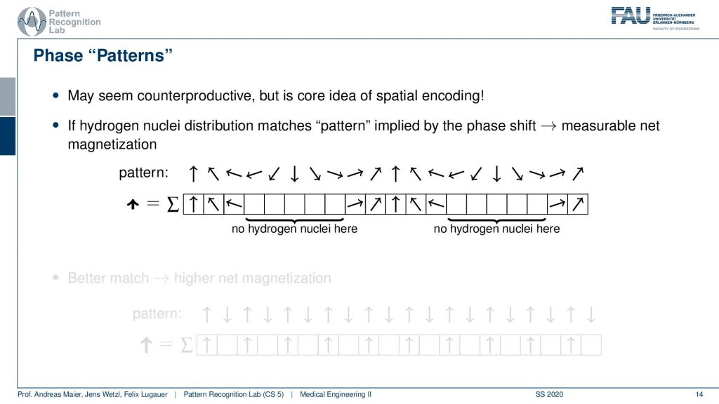
So you could argue that if I have a pattern then I can essentially interpret it as I’m tilting them into a different direction. If I would not have any hydrogen nuclei here then I would not measure this part of the signal right. So I would only measure the hydrogen nuclei that are essentially in phase here. So you could say that if I have a certain spin, then this gives me a pattern of rotation. By measuring I kind of measure the agreement of the magnitude of rotation with the actual observation here. You see that we will get a higher agreement if we have a better match. 

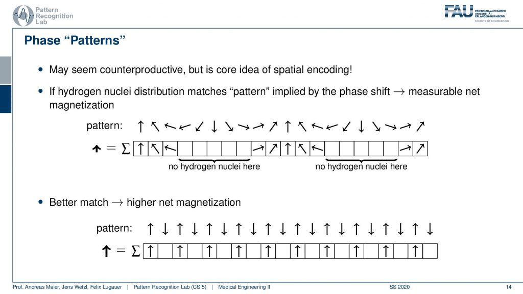
So if my underlying pattern is this here and I have this kind of orientation in my actual signal, then I get a very high excitation. If the match is not so great I get a lower agreement. We already described something similar when we are talking about the correlation of signals. But let’s make it a little clearer. 

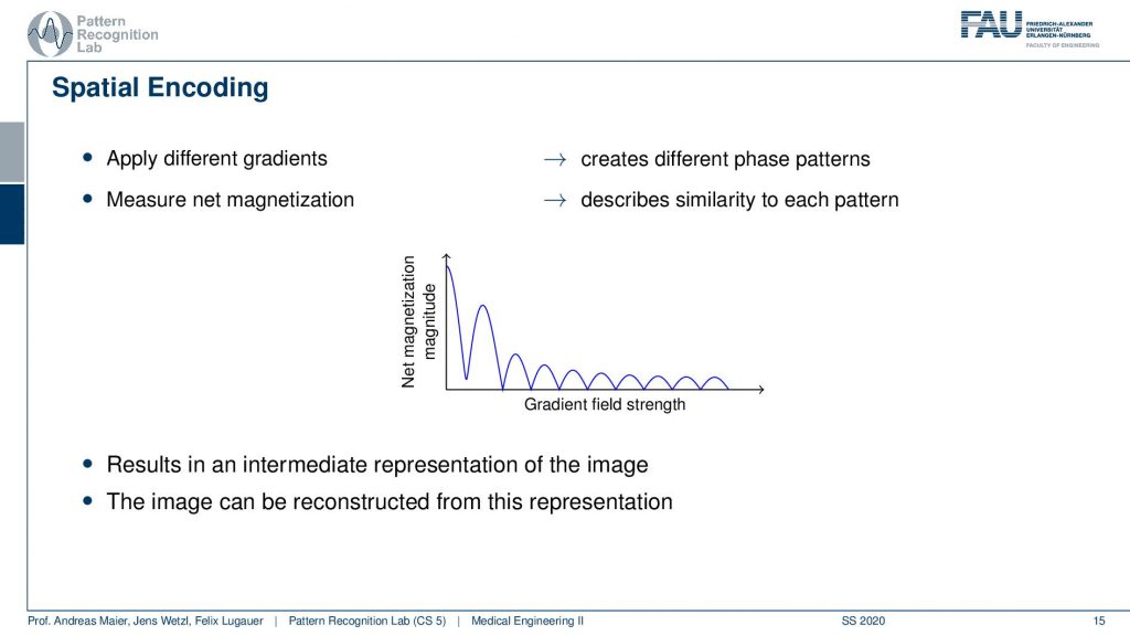
So what we are essentially seeing here is the agreement with the kind of phase shift along with the gradient field strength and how strong this agreement is. You see this is this curve here. So if we apply different gradients, we kind of apply different patterns, and by measuring we pointwise multiply them and add them up. So this is describing measuring the similarity between the pattern and the extra voxel configuration. Now I get this trace and the trace here describes essentially how the strength of the different orientations is encoded in the actual voxels and actually this guy here is an intermediate representation of the image. So if I know this trace I can reconstruct the entire information that was in my set of voxels. How? Well, let’s think about this a little more. 

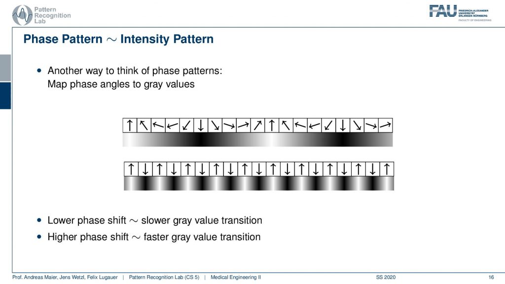
So what we actually have is not just the binary patterns as we’ve just seen but you can think of this as a kind of intensity pattern. So you could say here I have a strong orientation towards the top, to the bottom, to the top, to the bottom, to the top. So I could also encode the gray values in the following way here right and you see we kind of get this sine wave. If I have a fastpitch then I’m essentially getting such a kind of signal. So we get a sine wave with a very high frequency. This is interesting now we have these waves coming up here but as intensity patterns. If I have a lower phase shift then I have a slower gray value transition and if I have a higher phase shift I have a stronger gray value transition. 

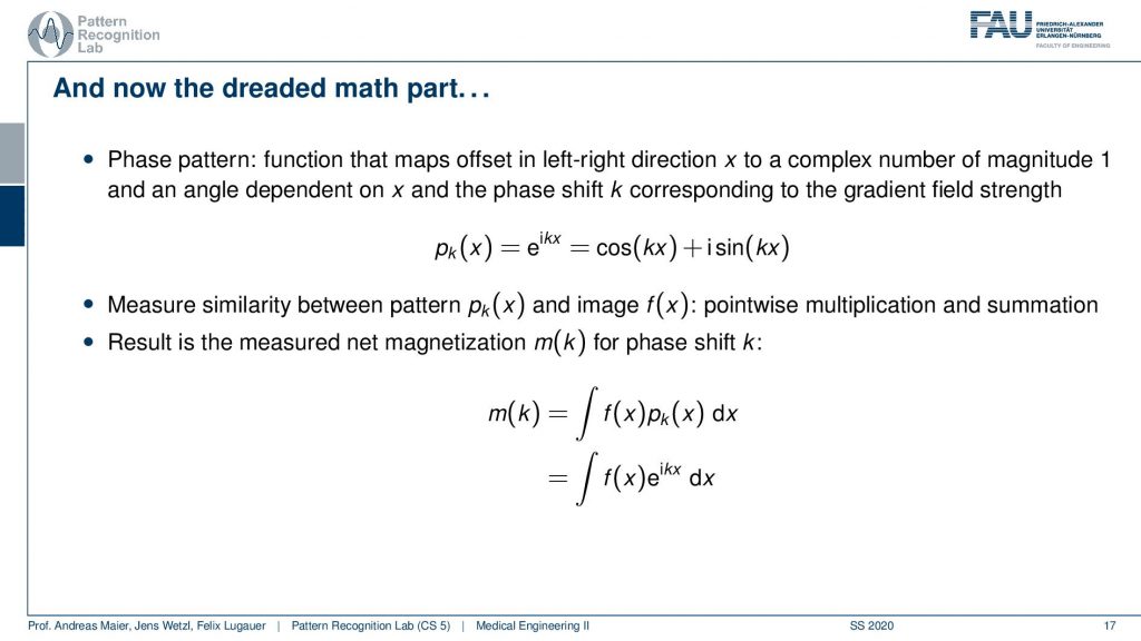
So what then happens is that two signals I can actually describe as sine and cosine signals. So our phase shift here can be described as this complex composition of sine and cosine waves. Now you can already figure that out what we are measuring is integral. So this is essentially the sum of the signal point-wise multiplied with each other and then all of the sum term. So we have this e to the power of ikx times f(x)dx integral. We’ve seen this guy before right striking similarity. 

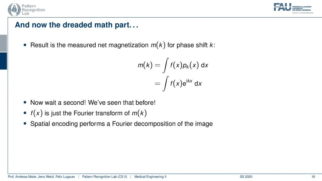
What we measured here is exactly this integral of a sine wave with the actual function that we seek to measure. We’ve seen this before f(x) is just the Fourier transform of m(k). So what we are actually measuring is the Fourier transform of whatever we want to reconstruct. If we know that we have the Fourier transform we can apply the inverse Fourier transform and then we get exactly our f(x). So the MR measurement does nothing else than acquiring the Fourier transform of the image that we want to reconstruct and the inverse v transform then gives us the original image. 

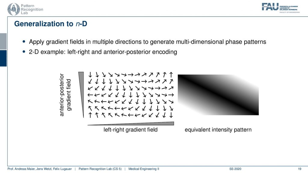
Now obviously what we’ve seen so far is only a 1D example. Now obviously we can also do this kind of gradient orientation with a 2D case. Then you get a gradient in the x and y direction and if you’re superimposing these gradients what you actually end up with is a kind of plane wave. So you see that we now have oriented waves here and you could see that this is a kind of plane. You see all of the valleys and so on they are aligned here. So we’re getting a kind of plane wave and if I play with the gradient directions I will be able to rotate this plane wave and I will be able to adjust the frequency or wavelength of this wave. This can be applied with the different combinations of the gradient coils in 2D directions.

Now if I do that then I end up measuring n-dimensional Fourier transforms. 

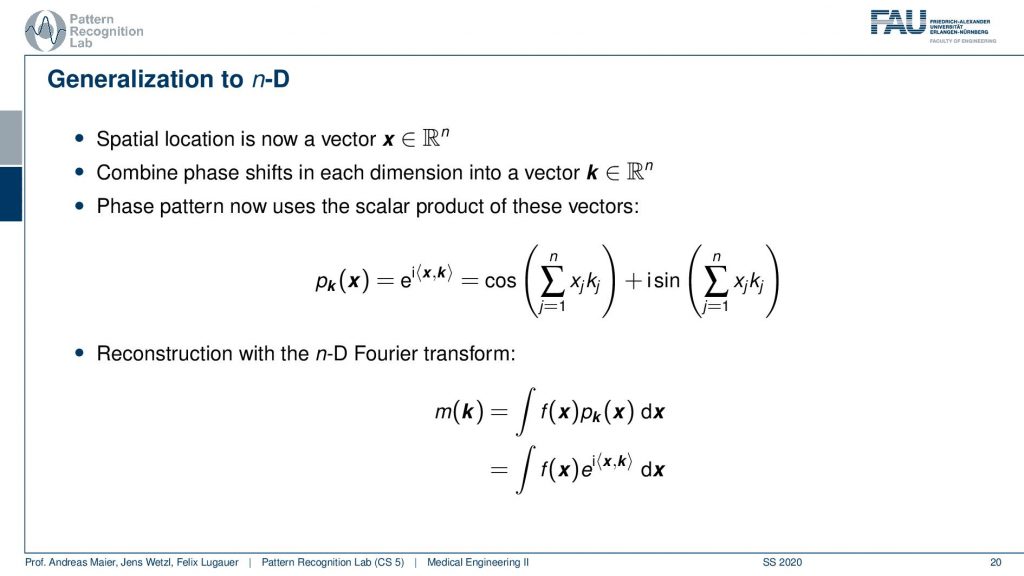
So I suddenly get now a scalar product and it’s the orientation of your wave and the inner product with the actual configuration at this voxel. Then I can measure the phase pattern in that way and this then leads to n-dimensional Fourier transforms. 

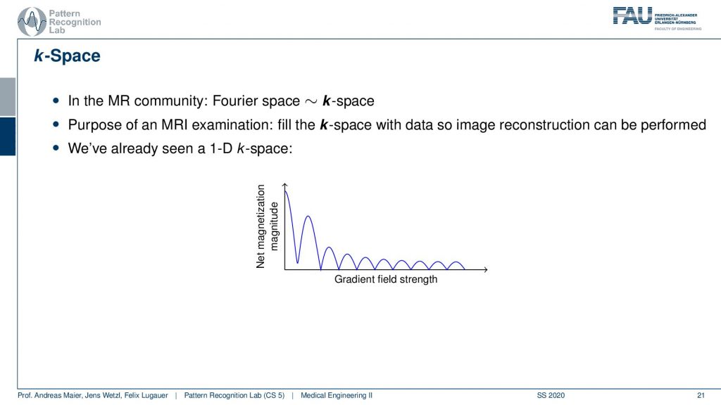
Now let’s talk about the so-called k-space and the k-space is essentially typically a 2-D generalization of 3-D generalization of that. So this is a 1-D space here and this is the 1-D Fourier transform of the actual image. 

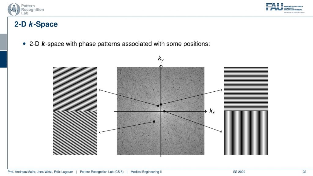
In 2-D the whole thing looks like that and we’ve already seen that when we talked about the Fourier transform in the image processing. So here space again is characterized by the orientation of our wave. So the k is the wavenumber by the way. So we can essentially determine the orientation. If you have a point here then you see that the wave is oriented in this direction. The distance to the center encodes the frequency. So the closer you go to the center the more you will have distances between the valleys and the hills. So this is a longer wavelength and now if I go towards something like this is may be oriented in this direction. Then you see that I have a high frequency here and that this is a wave that is oriented in that particular direction. So here it is the orientation direction. Then the further I go to the outside you see here you have already pretty high frequency. You see that this is essentially oriented in this direction and we also see that it’s further apart from the center. So the frequency is also higher. Now what I actually measure is this kind of signal pointwise multiplied with the image that I want to measure and then I sum up the entire field here and write this value here. If I want to measure this point here I take my input image multiply it with this image sum everything up and write it into this value. If I want to measure this point I take this kind of plane wave multiply it with the entire image pointwise sum it up and write it here and to compute this point I’m summing up everything multiply. So first multiply point-wise with this plane wave summing up and write it here. So this way you can construct a 2-D Fourier transform. So maybe if you haven’t understood the concept in the previous video maybe this helps to understand the 2-D Fourier transform. If you want to reconstruct this image what you take is for every pixel. Let’s say this is your image. This is what you want to reconstruct. If you want to reconstruct this pixel here what you have to do is you have to take essentially all of the points of the Fourier transform, multiply them with the corresponding plane wave(all of them), and then you look into this position and then you sum them up here. This gives you this result. So if I want to go from the Fourier space I essentially have to instantiate all of these plane waves and multiply them with the respective coefficient and then I sum all of them up in order to form the original image. So this would be an inverse to the Fourier transform. So we always need this kind of basis in order to construct it. Going 2 for your space is taking one plane wave multiplying it with the image here and writing it into the vector. On the other hand, going back is taking all of the points here multiplying them with the respective base functions, and then adding everything up in order to get the image again. So this is how you construct a 2-D Fourier transform in its inverse.

Very well! Now that we are able to measure all of these points of course we can also reconstruct them. 

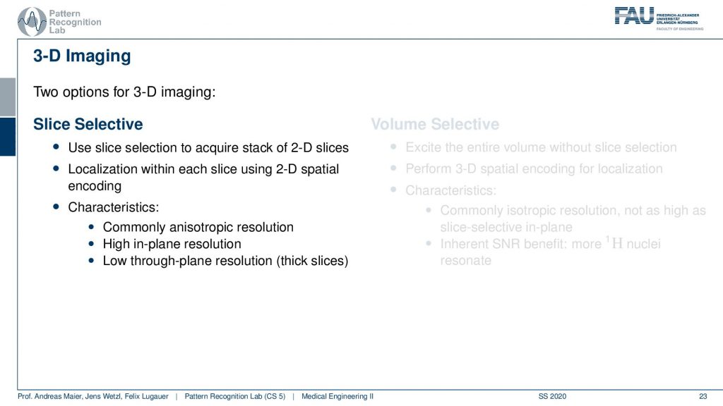
There is one more trick that you can do. instead of only using 2-D planes you can also excite entire volumes. So what we just discussed is the so-called slice selective encoding. I’m selecting slice by slice 2-D spatial sizes and then I compute the k space within this slice and reconstruct it. 

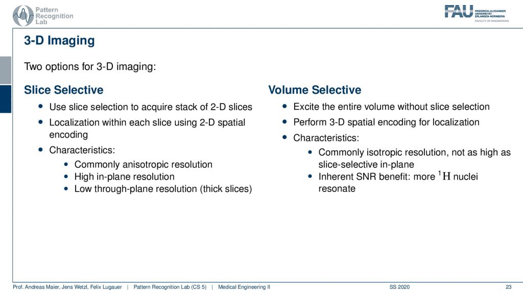
In contrast to that, you can do the volume selective one and there you encode essentially a 3-D k space. So now you take all of the three gradients in order to construct the brain waves. You don’t need the slice selection. Well, we probably still need some slice selection. But you know it’s a volume selection part because you’re computing the entire volume. So you excite in every step the entire volume then you perform 3-D spatial decoding. So we now have three orientations of the plane waves that also means that you have to acquire more of those points right and more of the orientations because you’re now sampling a 3-D k space. But if you think acquisition wise if you have the end slices or directly the 3-D k space maybe not so much different. Then one characteristic that you typically get is you get the isotropic image resolution and you have an inherent SNR benefit because more nuclei are excited and resonate. But obviously, you probably have more excitation to do because if you want to have an isotropic resolution you have to choose the same number of slices in every direction. Otherwise, the resolution will not be isotropic. So this then means that you probably also have to acquire for a longer time if you don’t have any kind of differences in the resolution in that direction. So this is why quite commonly these nice selective ones are used because then you choose thicker slices in one direction and then sacrifice this for scan time. So that’s the difference between volume selective and slice selective. Very well! Now you heard about essentially all the basic imaging techniques and we learned that our friend the Fourier transform is a very important feature here.

Then we can go on towards advanced applications.

The advanced applications that we want to discuss are going beyond simple morphological T1 T2 protein density imaging as we discussed in the last video. Then we also want to look into spectrally selective excitation and there you can use for example T2 preparation pulses and water-fat separation. Or you can go towards functional imaging where you then use non-contrast angiography of BOLD image, very advanced techniques. So let’s continue talking about this and the first thing that we will talk about is the T2 preparation for example for coronary angiography.

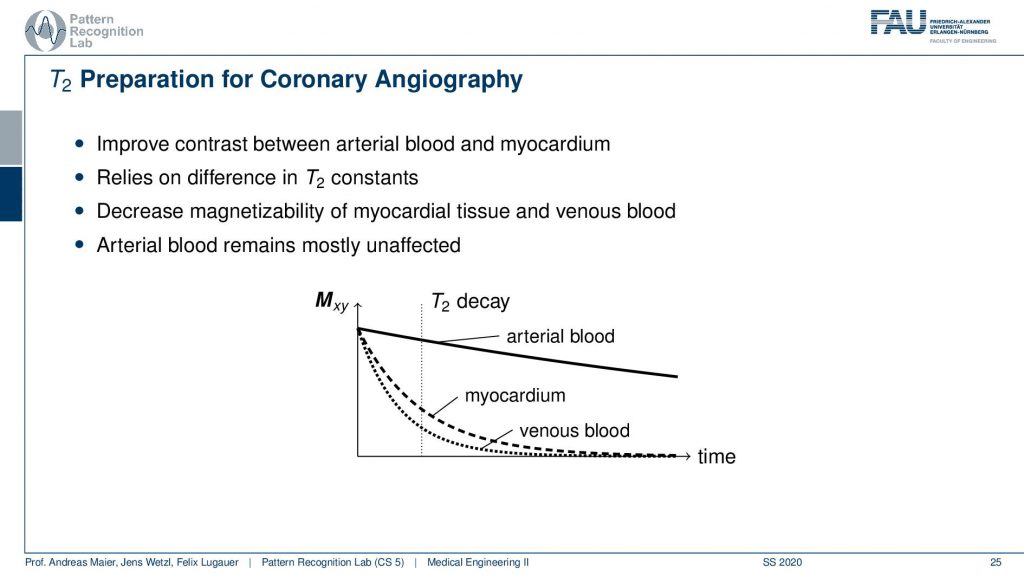
So there you want to improve the contrast between the ethereal blood and the myocardium and this relies on the difference in the T2 constants of the two. So there’s actually a change in T2 if you have arterial blood and if you have blood that is venous. This allows us to play with those effects and what we want to do is we want to decrease the magnetic size-ability of the myocardial tissue and the venous blood. This can be done by using the T2 decay. So we want to have the arterial blood to be mostly unaffected because the arterial blood has a much slower decay in terms of the transverse direction. This can be achieved by using an appropriate preparation pulse. Now if you do that then you can get images like this one.

So If you have a T2 preparation pulse you get the image on the right-hand side and if you don’t do that you get the one on the left-hand side. You see that the contrast is just much better on the right-hand side and you can really see the arteries in a very good fashion. So just in case, you don’t know where to look at it. So here you see the coronary arteries and you see that here we actually have arterial blood. In the ventricle, we have here venus blood and you see that the contrast is actually going down and we have this very nice preservation of the contrast here of the arteries and on the left-hand image you can’t see it as well. So this is a big advantage if you can work with this T2 preparation for getting better coronary images. 

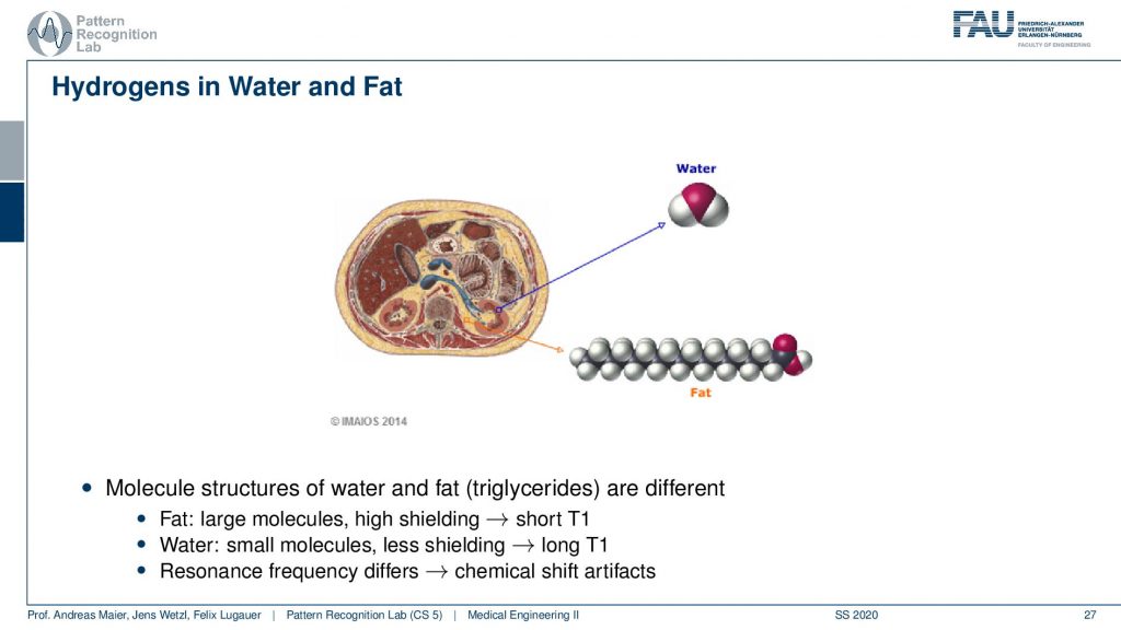
What I already hinted at is that there is a difference in the local magnetization depending on the type of molecule that the hydrogen atom is actually in. So you can see if you have water then our hydrogen is not in a strong binding. But if you have fat you see that there is a very different local magnetic field. So in fact you have large molecules and higher shielding and this means there’s a short T1. In the water, you have small molecules and less shielding. So you have long T1 times. This means that the resonance frequency differs and this is then called the so-called chemical shift artifact. So there is a different resonance frequency in fat than in water and we can use this effect to actually separate the two. 

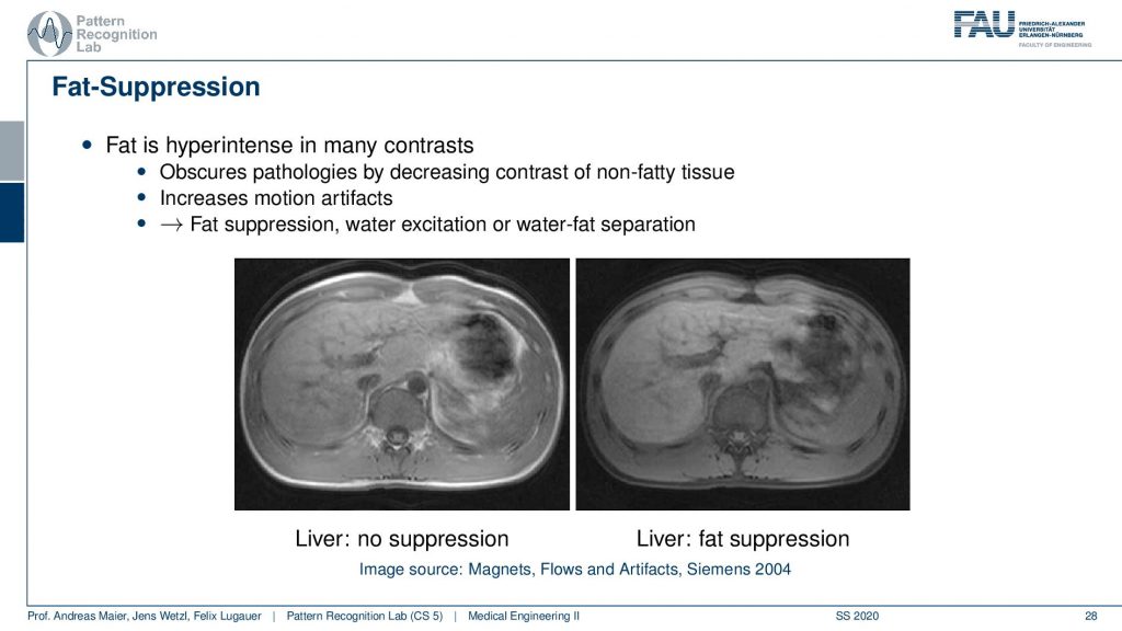
So this yields water-fat suppression sequences. If you don’t apply a water-fat suppression or fat suppression then you get images like this one here where you see actually a very strong signal in the fatty tissues here. If you have a fat suppression pulse then you see that this bright ring is gone and the contrast also remains mostly stable but the fatty tissues are not as visible. Now that you can generate this difference between the two. Then this allows for water excitation or water-fat separation. 

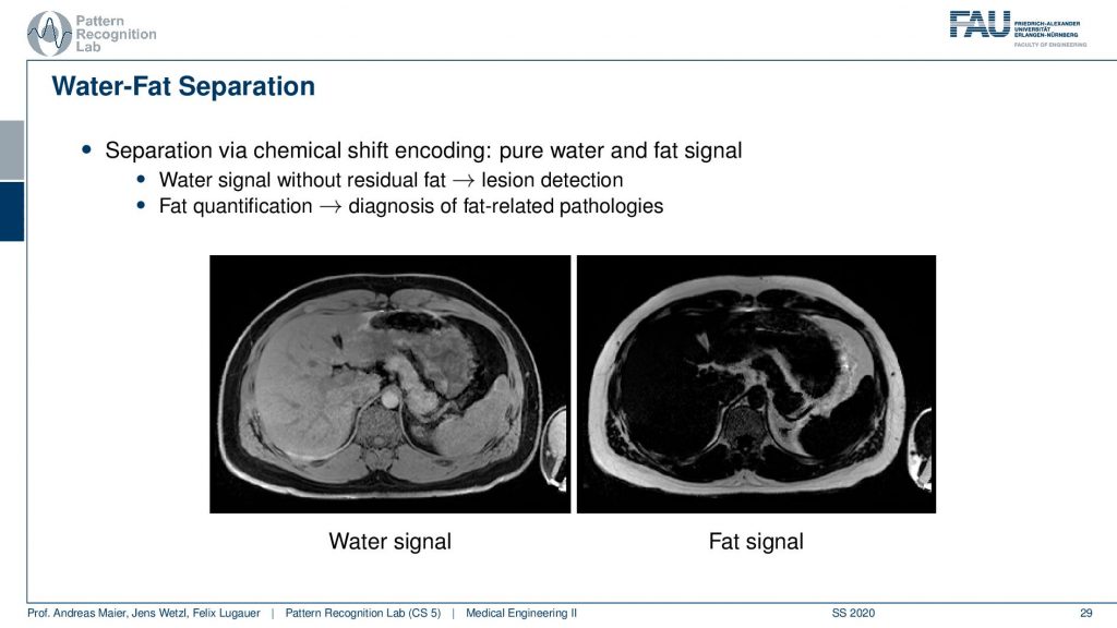
So an easy approach is then that you compute the water signal from this and the fat signal essentially by subtracting the two images. The fat-enriched and the non-fat enriched and this leads then to the decomposition into this materials. very well! Of course, this can also be used for advanced purposes. 

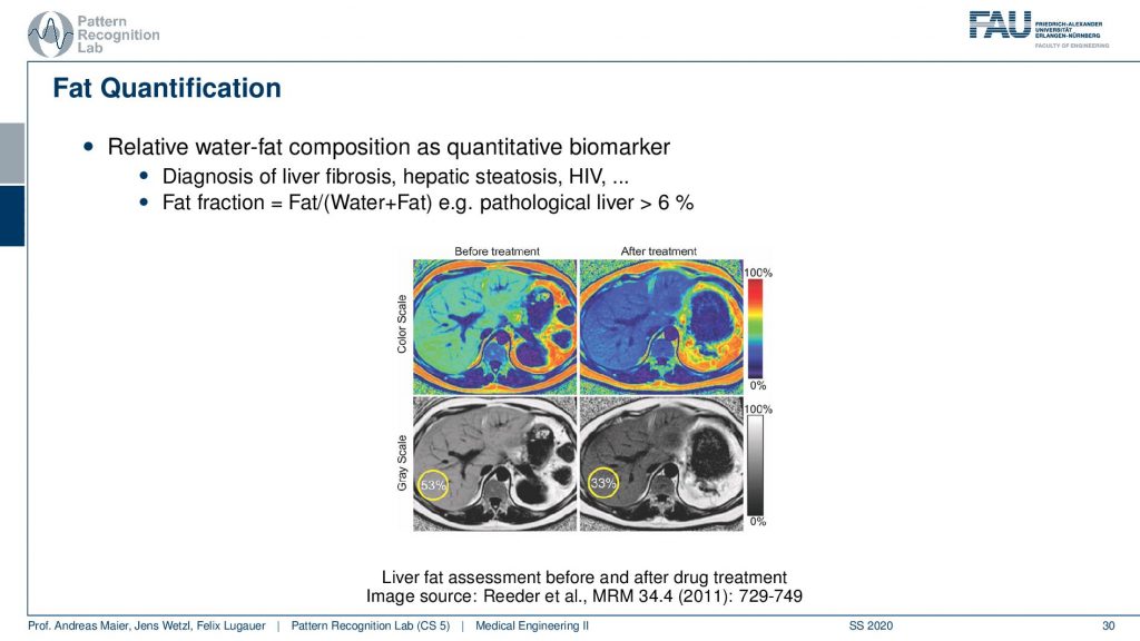
Here you can see that you can also then quantify the amount of fat in the tissues by these separation techniques. So it’s not just that you have pure water and pure fat in the voxels and they’re entirely suppressed. But you can also then compute the percentage of the signal in that respective voxel and this allows you to quantify really how much fat is in a particular voxel. With this, you can diagnose fat levers for example.

Let’s go to functional imaging and a very cool technique is the so-called non-contrast angiography.

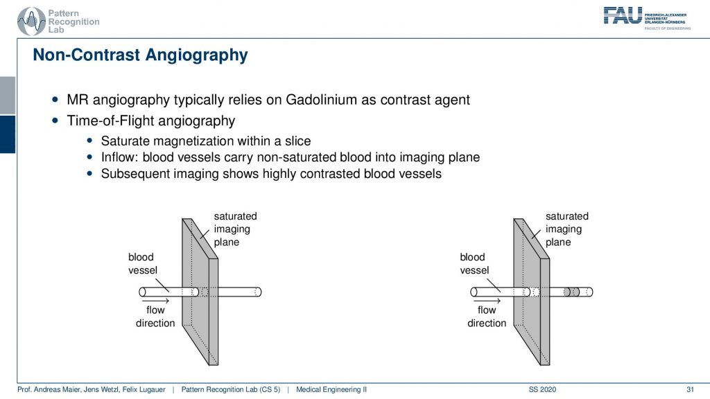
The key idea that is happening here is that you play with the actual imaging planes. So what you do is if you have a blood vessel and this is the flow direction. So you’re essentially exciting in this image plane and then you depend on the flow. So the excitation will have happened at this point but then you actually read out in this position here and that’s pretty cool. Because if you essentially change the gradient of the readout and this allows you to then detect whatever you are excited about here in this plane. So you use a different encoding scheme for the time of the readout. This is giving you then images that will only be able to read signals in this direction. That’s pretty cool because then I have magnetically kind of tagged the blood and the blood vessel but I don’t need any additional contrast agent. It’s not like that I have to insert iodine or gadolinium or something like that. I just use the magnetic properties of the blood itself and the excitation of the spins as a marker. Then very shortly I read it out in a different position and the only thing that is magnetized and in that particular slice is going to be the blood.

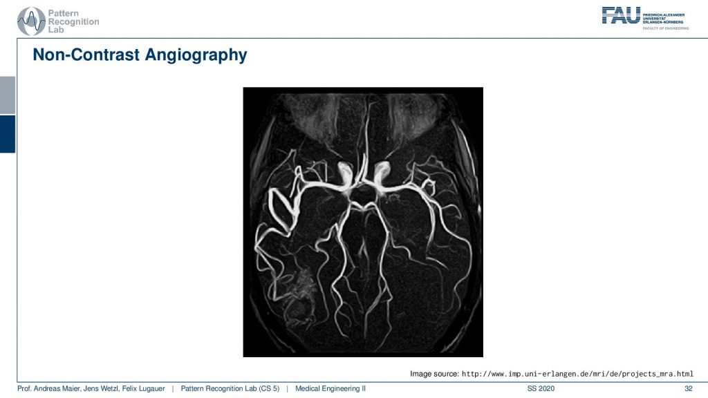
So this then yields to very nice images and here you see a visualization of brain vessels and this hasn’t used any contrast agent at all. You just use a kind of magnetization plane and then you measure in other slices the magnetization of the signal. So this is completely contrasted agent-free and that’s of course very good for the patient because they don’t have to inject the additional contrast agent. 

So there’s more to that. 

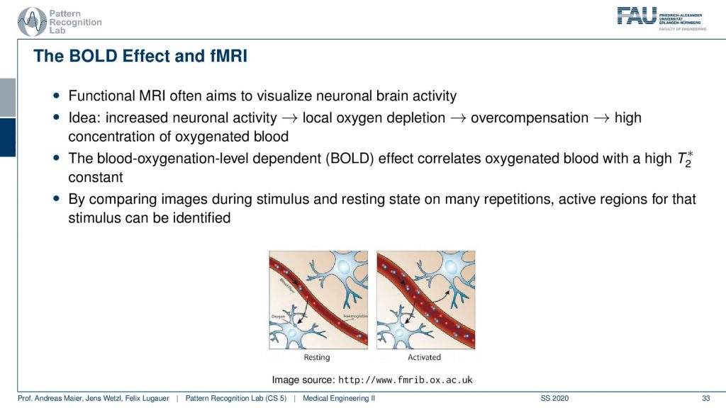
There’s also the so-called BOLD effect and this is a key technique for functional MRI. Here we essentially use the effect that we can also measure the blood oxygenation in a similar way as we’ve already seen that for differentiating arterial and venous blood. The MR contrasts are dependent on the amount of oxygen in the blood. If we know that we can actually measure the areas where there is more blood or less blood in the brain. This works at a rather short time frame. So it allows us to figure out in which areas of the brain more blood are deoxygenated and this allows us then to figure out which areas of the brain are active. This is of course a key tool towards understanding the brain in neuroscience. 

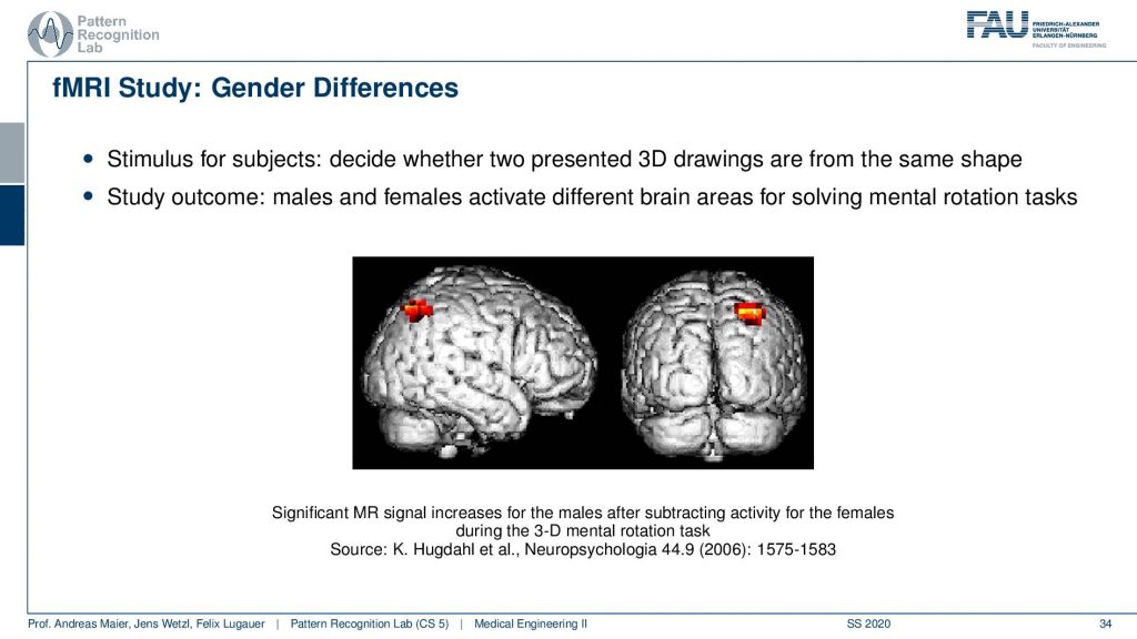
So if you look at that you can then generate maps like this one where you have a visualization of the brain and then you show a certain stimulus. With the stimuli, you can then figure out in which areas of the brain the most signal loss was taking place. This allows us to understand where actually the oxygen in the brain was used. This is essentially indicative of metabolism in this area and this then allows for figuring out which parts of the brain were active. So if you then visualize these things what is happening quite often because the signal is rather low. It’s not like that you can just pinpoint for a specific individual where the actual oxygen was used. But you need to do many measurements and then what’s often done is that you average over groups. Here you see that this is an average over males and females and here they could identify a certain area that was activated differently in males and females for specific stimuli. So here you have actually the difference during a 3-D mental rotation task. So in a 3-D mental rotation task, this particular area of the brain is used in a different way between males and females. So a very interesting technique that has been used very very frequently in order to understand the brain and to get better insights into neuroscience. There are more. There’s also diffusion-weighted imaging. In diffusion-weighted imaging, you can essentially figure out the orientation of the Brownian motion inside a volume and this then allows us to estimate fiber directions for example in the brain. This leads to the field of connectomics and connectomics is used to reconstruct the connections between the different brain areas. There are indications that in specific diseases the connection between the areas is changed and therefore the connectomics may be indicative of certain neurodegenerative diseases.

Very well. This already brings us to the end of this presentation. So now you’ve seen also how we apply imaging in MRI. You’ve seen that we are essentially changing the gradient coils in order to introduce changes in the magnetic field that are locally different. We can use that for slice excitation. So with that, we can read out a specific slice direction and only the voxels within the slice are excited. Then we can read them out. In order to figure out in which location they actually are we use an additional gradient before the readout to introduce a phase shift. With the phase encoding, we could then interpret this as a kind of plane wave that is multiplied with all the exciting voxels of that particular plane. When we read out the signal we are reading out the multiplication and the sum over all of these boxes. This we could demonstrate to be identical with an inverse Fourier transform and therefore we can use the Fourier transform to reconstruct the measured image. So you can see that with these very elegant steps we are able to actually obtain image information from arbitrary plane directions. So you see this is a pretty cool effect and with this, we are able to measure very elegantly the entire human body and arbitrary orientations without any ionizing radiation. Yet we’ve seen that the disadvantage of this effect is that it’s pretty slow. In particular, if you have demanded that you need images very quickly you might want to use other kinds of modalities. In particular, we want to start in the next video talking about x-rays and they are very very commonly used in particular in emergency situations but also for acquiring bone and soft-tissue contrast. So this is what we’ll start talking about in the next video. Thank you very much for watching and looking forward to meeting you in the next video, bye-bye!!

If you liked this post, you can find more essays here, more educational material on Machine Learning here, or have a look at our Deep Learning Lecture. I would also appreciate a follow on YouTube, Twitter, Facebook, or LinkedIn in case you want to be informed about more essays, videos, and research in the future. This article is released under the Creative Commons 4.0 Attribution License and can be reprinted and modified if referenced. If you are interested in generating transcripts from video lectures try AutoBlog

References   

1. Maier, A., Steidl, S., Christlein, V., Hornegger, J. Medical Imaging Systems – An Introductory Guide, Springer, Cham, 2018, ISBN 978-3-319-96520-8, Open Access at Springer Link

Video References

1. The Entertainer https://youtu.be/aQQ-Azi26N4
2. Fast Spin Echo Animation https://youtu.be/RI-YtEBcHkc
3. 2D Fourier Transform Example https://youtu.be/js4bLBYtJwY
4. MRI Angio Brain and Neck Vessels https://youtu.be/7EGKe3u5sMI
5. Randy Dickerson – Syngo Via VB20 Cinematic Rendering https://youtu.be/I12PMiX5h3E

Category: Lecture Notes in Medical Engineering