
These are the lecture notes for FAU’s YouTube Lecture “Medical Engineering“. This is a full transcript of the lecture video & matching slides. We hope, you enjoy this as much as the videos. Of course, this transcript was created with deep learning techniques largely automatically and only minor manual modifications were performed. Try it yourself! If you spot mistakes, please let us know!
Welcome back to Medical Engineering. Today I want to discuss with you the properties of magnetic resonance imaging. So we will revisit the basics of MRI. We will look into the physics, we will try to understand what magnetic resonance is I have a couple of very simple examples to show you how this effect emerges. Then I want to gradually go ahead and describe how we can use the magnetic resonance effect to measure the physical properties of tissues inside of the body. So this will be a video that is split into two sessions. In the first session, we will talk about magnetic resonance and how the effect emerges, and how it can be used for measurement to differentiate different tissues and their properties. In the second video, we will talk about magnetic resonance imaging. So there we want to think about how we can use the signals and resolve them into an image signal. So looking forward to exploring medical imaging and magnetic resonance imaging with you guys.
Magnetic resonance imaging magnetic resonance effect: So the technology that I want to show today is rooted in basic magnetic physics. You will see that varying magnetic fields then also are related to electromagnetic radiation. So we will look into those effects and we will see why we need varying magnetic fields to be able to express how the actual physical effect emerges and how we can use it to figure out something about the images. So first we’ll look into the genesis of the resonance effect and then we look into how we can use that to figure out relaxation and contrast.
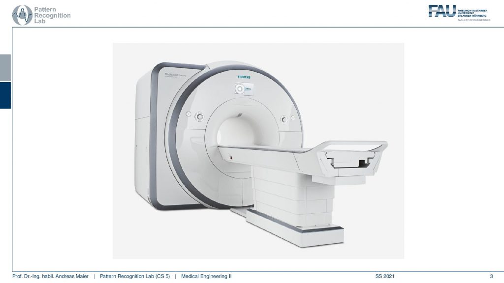
So let’s start this is an MRI scanner. It is a huge you could say donut-shaped kind of device and you can see that in contrast to a CT Gantry the hole is much deeper. So the devices are much longer. You could say that the hole is probably two meters long. So if you look at this patient bed approximately as long as the bed is the scanner also extends to the back. So you see the magnetic resonance imaging devices are bigger heavier can weigh several tons and typically they are located in the basement because they are so heavy. Now, why are they so heavy? Well, one of the key elements of a modern MR scanner is a superconducting magnet. To have the superconducting properties, the electromagnet has to be cooled down and it has to be cooled down close to absolute zero not entirely but way beyond minus 150 degrees Celsius. So you need a coolant that can reduce the temperature of the magnet to such low temperatures for example liquid nitrogen is one of the coolants that is used here. So what you see in this kind of scanner is this kind of donut shape and then there are magnetic coils, electromagnets built into the scanner. They are switched on and off to introduce additional so-called gradient fields to adjust the magnetic field. Then there is the huge scanner that is driven by the so-called B0 of the main magnetic field and this one has to be ramped up actually over a couple of days. So it’s not just possible to turn off and on the magnetic field although it is an electromagnet. It takes a couple of days to get the system operational. So also be very careful these magnets have a very very strong magnetic field. If you operate them you have to be very careful, first of all not to damage yourself anything that’s of metal might be accelerated by such a magnet. So there are pretty interesting videos that you can find on youtube about what actually happens with MR safety.

The other effect of course is that you have to be very careful not to damage the housing because there is liquid nitrogen in there or other very cool liquids. If you harm the housing then the first thing that happens is that they are connected to something that has room temperature. So they will very quickly expand and then rush out of the coolant system of the scanner. Then they very quickly push out the remaining breathing air out of the room and if you have stuff like nitrogen then you can very quickly suffocate. So what happens if there is an accident in such an MR scanner. One of the first things that you want to do is you want to lower yourself you want to go to the floor because the nitrogen will go up. Then you might be able still to breathe and you want to leave that room and maybe also the building as quickly as possible. Because once the coolant emerges that’s quite a bit mass that is emerging from there. So it’s very dense because it’s cooled and if the coolant gets to room temperature then it expands as a gas. So it will use much more volume than previously. So this is then called a quench and also if you have a look at youtube you will find amazing videos of MR quenches.

After having said that obviously it’s an expensive technology but it also has a lot of advantages over other volumetric modalities like CT which is X-ray-based.
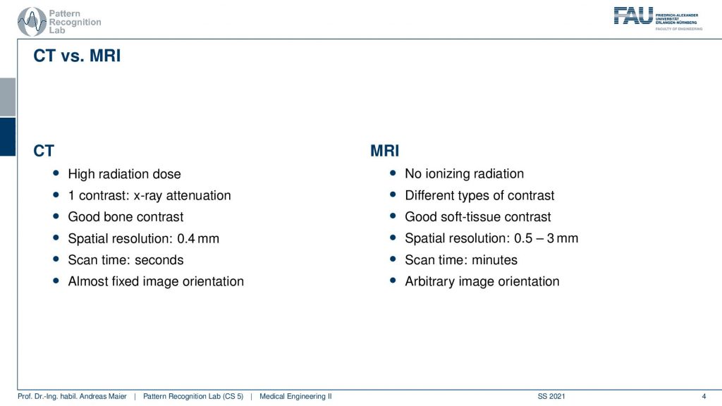
This we will get to know in one of the next videos. They have ionizing radiation. So it has a radiation dose that has the risk of breaking your DNA and this has a long-term risk of introducing cancer. So this is a big difference from MRI. So there is no ionizing radiation that is being used and it’s all based on electromagnetic radiation that is essentially in the wavelength of microwaves. The next thing is that the scanners have a very good contrast resolution. In x-ray scanners you can differentiate contrasts quite well in particular in CT you can differentiate bony tissues like the bones, the bone marrow, you can differentiate different organs but the contrast is not that great. It’s enough to resolve the brain and the skull and the fluids in the brain or different organs in the abdomen. But if you have MRI you can even differentiate gray and white matter. So it has good soft-tissue contrast. This is also one of the reasons why the technique became so popular. The spatial resolution is different in ct you have a very fine spatial resolution. So we’re back to the trade-offs that we’ve already seen. Special resolution in ct is approximately 0.4 millimeters in MR you have 0.5 millimeters to up to 3 millimeters. In MR the resolution is essentially proportional to the scan time in ct to the radiation dose. So if you would want to increase the resolution you would probably have to increase the dose in CT and MR they just scan longer. This brings us to the next feature of those scanners. A CT scanner can scan the entire body in up to 10 seconds in MRI it may be minutes and it’s not uncommon that you stay in an MR scanner for up to half an hour if several protocols are acquired. So this is something that is a clear drawback of MRI that the scan time is much longer. But of course, it has also many advantages and this is why it’s very popular still in diagnostic imaging. So in CT, you have a fixed orientation because the orientation is essentially determined by the physical properties and the gantry orientation of the system. We will see that when we talk about the modality. In MRI we have the gradients and the gradient coils that can essentially be freely programmed so we can acquire images at arbitrary orientations. So in CT, you have to cut along certain planes and you can only reconstruct within this plane in MRI you can place planes in any kind of orientation as you like. So that’s a huge advantage.
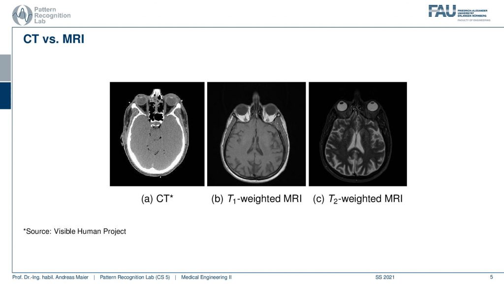
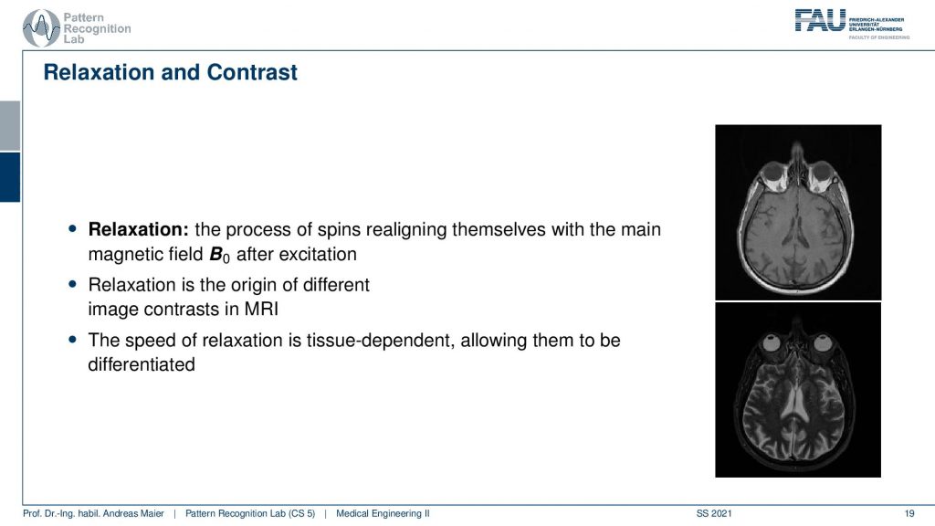
I have a short comparison here of these different contrasts that can be reached. On the left-hand side, you see a typical ct image where you see the bones very well. You see that there is a brain inside but it’s hard to differentiate the different tissues. In the center and right image, you see two different contrasts that can be obtained with MRI. So you see one big advantage is that you can program essentially sequences that generate different tissue properties like here the T1 and T2 waiting. We will see that towards the end of the video what that means. The next thing is that we can see soft tissue. So here you can see that the gray and white matter in the brain can be seen in the two different images. You can also see is that we kind of see the skin that is on the outside of the skull. But we get no signal in the bone. So MRI is not very good for imaging bones. So everything that can be seen well is associated with high concentrations of water. So this is also a special property of the MRI imaging system.
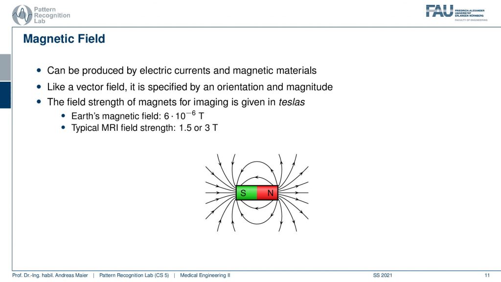
Now that we’ve seen the idea of the contrast and why it makes sense to actually work with such an MRI system. Let’s look into physics. The physics of MRI is based on magnetics. The magnetic field that you probably know best is the earth’s magnetic field and most of you have already seen a compass and the small needle that is also a small magnet. This magnet then aligns with the earth’s magnetic field. So you see here the north and the south pole of the earth magnetic field and then you can see that the compass needle will start aligning with the field if you for example turn your compass. What will happen is that the needle will not directly assign with the compass direction. So with the main magnetic field but it will actually overshoot the main direction and after overshooting it returns and returns and you can see that with every swing the magnitude is reduced. But the time it takes for each swing is constant. So it has a fixed frequency and it tends then to orient with a stronger main magnetic field.
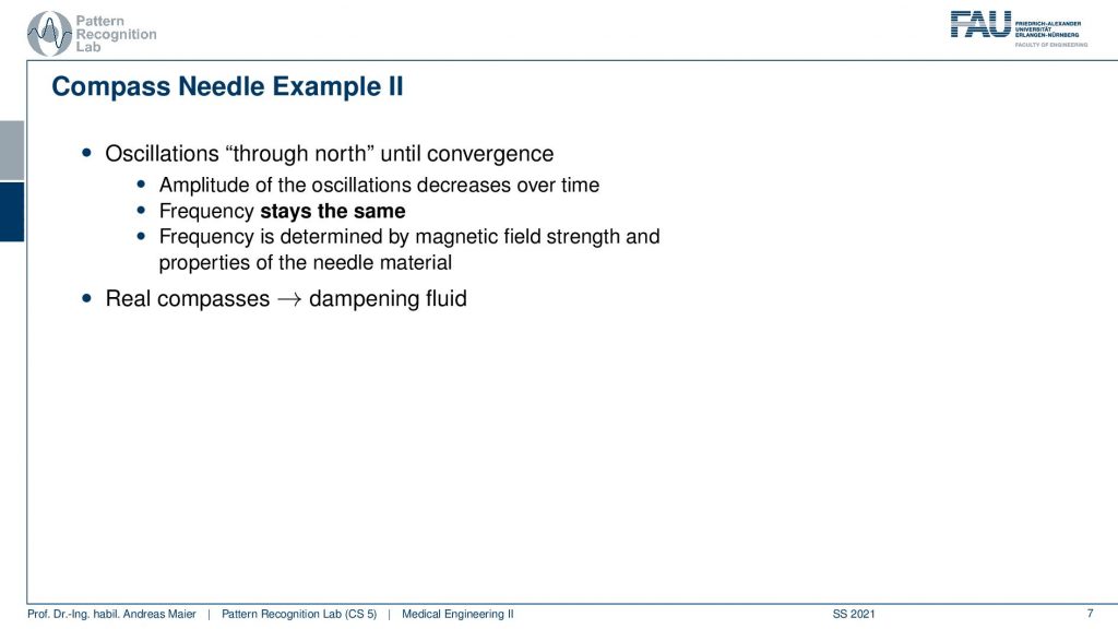
So we can now observe that the oscillations through the north will repeat until convergence. So the amplitude will get smaller with every swing and the frequency stays the same. This is a key concept that we will use actually in the imaging that the frequency for this oscillation remains the same. Now the frequency is actually determined by the magnetic field strength and it essentially gives us some information about the properties of the needle material. In a real compass, you won’t observe this effect as pronounced because there’s typically a dampening fluid in there such that the oscillations are not as strong. You can see that the needles that we have or the small magnets are also influenced by their surroundings so here the dampening fluid. You will see that similar effects will also occur inside of the body. So it’s not just that we measure the presence of small magnets but they also are embedded in their surroundings. Therefore we can also measure with MR systems not just the properties of the magnet but also there you could say microclimate.
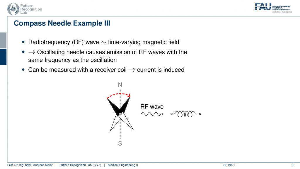
Now what happens here is if we would like to excite our magnet then we would have to somehow tip it in the right frequency, right? So if I want to get the needle back to swinging I essentially would have to take a magnet and push it and at some time I remove the force and then I push it again and remove the force and if I do that in the right frequency I can actually manage to get the needle oscillating. If you now have a changing magnetic field that is actually equivalent to a radio frequency wave. So whenever you have an oscillating magnetic field it immediately associates with radiofrequency waves. Then there are typically also these radiofrequency waves being emitted.
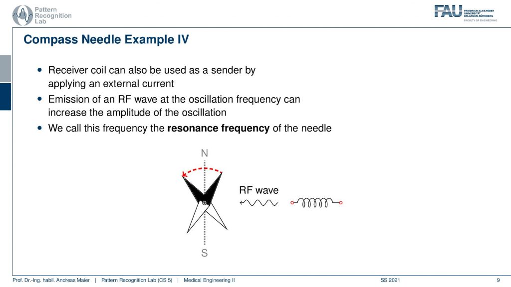
So the idea now is that we have the small magnet and if we push it excited and get it to swinging then we can stop pushing. Then we can measure how it returns to the main magnetic field. So this is the key idea of magnetic resonance imaging. So this will later then give us the contrast. So we push the needle somehow, we’ll see that’s an rf wave and then we stop the rf wave and we can measure the rf wave that comes out of the needle later this will be the tissues. We can therefore determine something out of the properties of this needle. So it tells us something about the property of the needle and this is essentially the main idea.

I have a small example here for you and you here see the URL and I have this here open on my computer screen.

Now, this is the magnet needle and you should be able to see my mouse cursor here. This is the needle and I would like to push it. Let’s push it there. You push then you see that it starts oscillating and after some time it will return to the original orientation. Now what we would like to do is we want to excite it right and I said that we want to take a magnet and if I take a magnet and bring it close. You see that I deteriorate the main magnetic field with this additional magnet. I’m able to push the needle here to the side. Now if I remove it you can see that it quickly returns to the original orientation. So if I want to get this needle swinging strongly I need to go remove it and then push it back. You see if I appropriately do this then I’m able to tip this needle pretty far. If I tipped it pretty far you can see that it then takes a longer time to return to the equilibrium state where it is aligned with the main magnetic field. Now, this is hard to do you know I have to be at the right timing and then I have to return here to kick off the needle and this is maybe not that great. But I could push this at a certain frequency. So let’s do this automatically so I take my magnet and bring it back in. Here is my magnet and now it’s swinging for me. So I configured a frequency here and it’s automatically running back and forth now. You can see I’m a bit too quick with the frequency. So maybe I want to reduce the frequency a little to bring my magnet pushing this needle you see yeah that’s appropriately a good frequency. Maybe I want to introduce a higher field strength. But you see how I can push it off and maybe I’m just a little bit too fast. So I think this is better now you see how we can tip it very nicely. Now instead of taking a magnet and moving it on and off again or two and back of the needle, I can replace this with a coil. This is an electromagnetic coil and now I change essentially the polarization of the coil all the time. This enables us to get a constant oscillation here for our magnet and you see if I now turn the magnetic field off then there is a resonance. You see the resonance here and the resonance is being plotted in blue. It slowly returns but it has a constant frequency. So if I turn it on again you see I’m able to excite it so I’m essentially sending a radio frequency wave to our small needle. Then I turn it off and you can see how the oscillations dampen at a fixed frequency and how it returns to the equilibrium state. So this is already the key idea of MRI imaging. So we are actually generating an RF part in the right frequency. I can also show you if they take the frequency too high then you know nothing happens big, right? If I turn this off now you see that there is no oscillation. So I have to pick the right frequency and maybe this frequency range in order to get the excitation. You also see the better I manage to get the right frequency the higher actually the excitation will be. Now you see that we have a pretty strong excitation. Now I turn the magnetic field off again and I get this very nice dampened sine wave as a result. So you see this is the key idea of magnetic resonance imaging and here we use then later this effect to measure what’s happening inside of the body.
Good! So why are we talking about the body there are no magnets in the body, right? So it doesn’t make a lot of sense.
Well, that’s not entirely true because the magnetic fields that we want to measure they can be part of very small dipoles of very very small kind of elements that you have in the body. In particular, you have something that is close to a small magnet and these are the hydrogen atoms that you have in your body. So hydrogen you could interpret as a small magnet. The problem is the magnetic fields are very low. So to be able to use the magnetic fields you have to make sure that the hydrogen atoms align inside of your body. The earth’s magnetic field is way too little. It’s not enough magnetic field to cause your hydrogen atoms to be forced into the main magnetic field direction. So it’s not strong enough. So this is why we can measure these effects in the human body as it is. So everybody of you knows you’re not unless you’re Uri Geller or somebody you’re not magnetic and you will not have a magnetic field.

So we somehow have to produce an external magnetic field that is strong enough and to do that you need high magnetic fields. So the earth’s magnetic field is something like 6 times 10 to the power -6 Tesla. So Tesla is the unit to measure a magnetic field. The earth’s magnetic field although it’s enough to tip a compass needle it’s way not enough to tip the hydrogens in your body. So what you need is 1.5 or 3 Tesla or in high field scanners 7 or 9 Tesla. Obviously, the higher the magnetic field strength is the more signal you can generate. Therefore if you have very strong magnetic fields then you’re also able to image quicker and also a smaller contrast. This is the reason why in high field imaging you can then also image other atoms than just the hydrogen. This can then also be applied to other kinds of molecules and atoms.
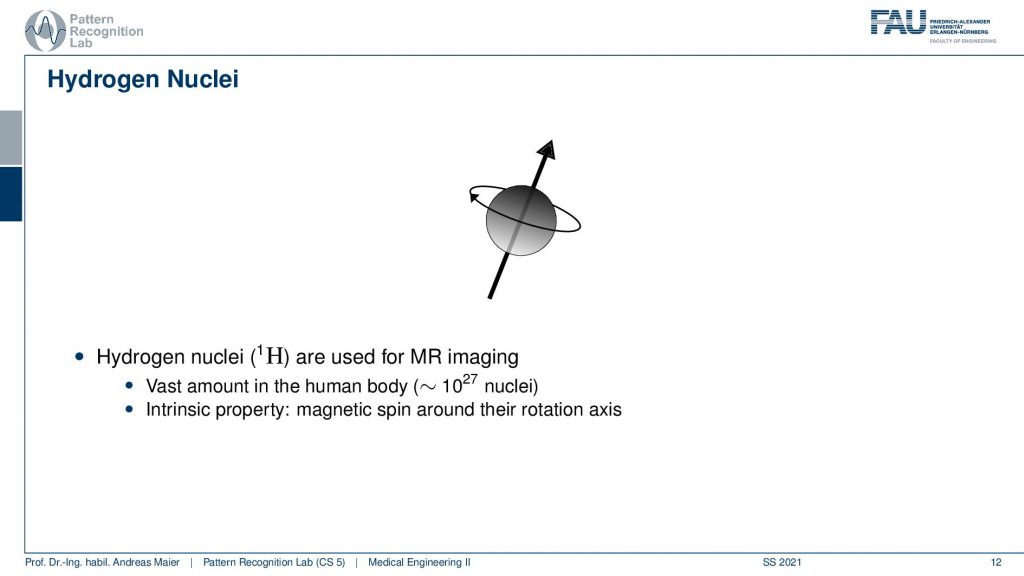
Now let’s have a look at some Hydrogen nuclei. A Hydrogen nucleus is essentially an electron that is spinning around the core and the core is typically made of a proton and maybe also depends on what kind of hydrogen you have there may also be neutrons available. But it’s one positive charge and one negative charge. The negative charge circles around the positive one and the plane of the circling defines essentially the orientation of your magnet. So we actually show this here with the spin and the actual orientation of the magnet in this image. What then actually happens is that you not just have one hydrogen nuclei in your body but you have many of them.
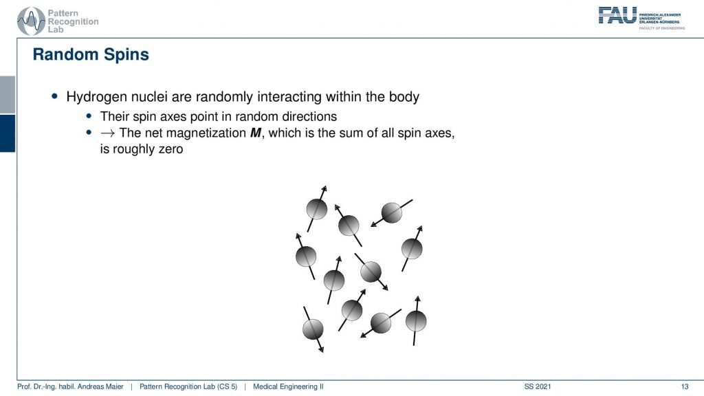
Typically they are not oriented in a particular way because the main magnetic field is not strong enough to orient them. So they are somewhere in your body and they are oriented with arbitrary orientation. The net magnetic field that emerges from that is simply zero. Just because they are randomly oriented all of the magnetic fields cancel out and you’re not magnetic as you already have noticed that your body doesn’t have effects on magnets and they don’t stick on your body. So this is the typical state that your body is in.
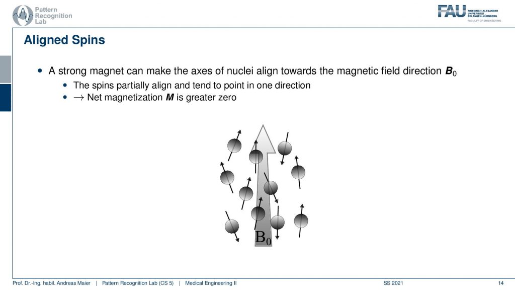
Now if you apply a strong external magnetic field what happens is that the same thing as we’ve just seen with the compass needle, the axis of the hydrogen atoms will align. Because they are aligned they will suddenly all be oriented either along the field or against the field. So you then have this effect that you have an alignment and it takes some time once you enter the magnetic field not too long but then all of the atoms will be aligned. If you have that then what also happens is that the magnetization is not just zero. But there is some additional magnetization that is found because all of the hydrogen nuclei align. They kind of flip into opposite directions but there is a certain tendency to more flip into the direction with the field than against the field. So there is now an additional magnetization and the net magnetization is there with greater than zero. Nonetheless, they are now all aligned and they can be excited.
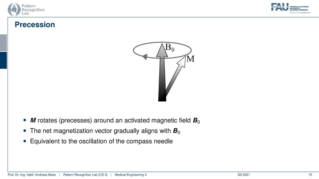
Now what happens is if you try to excite them it’s not like that these small magnets just tip. Because they are living in the 3d space, so they orient with the main magnetic field that is shown here as B0. As soon as you try to excite them they get into a so-called precession motion. The precession essentially means that then once they’re aligned with the magnetic field they’re probably here and then they start circling like this right and the more you excite them the more they process. Now this precession motion is a bit complicated to actually imagine it or to demonstrate it and I would have to play a lot of games of my pen here but I prepared a short video here. This is a nice video by the MIT department of physics and you actually can see it on youtube.

You will also find it in the example. So we’ll put it in the description. We don’t need the sound because there’s no sound anyway. So here we don’t have magnets but we use the gravitation field and now we have a spin. You could see that this the electron that is circling around the proton. Now we get the precession motion. So what will now happen is we excite this additional gravitational force and then you get this precession effect. So the spin is very very fast but the excitation has a certain rotation frequency. This is the precession frequency which is moving in a direction that is essentially perpendicular to the main gravitational field here. You can think of the effect in magnetization as very similar. So this is the precession effect and now you can see that we essentially have two main directions. We have the direction along the field and the direction orthogonal to the field. We kind of have this effect that circles around the main axis at a constant frequency. But you see that we are reducing the amplitude here as well. In the final state, the two axes will be aligned with each other again. So this is the main idea of precession.
Okay now that we understood what precession is then we can also see why we exactly have two main directions that we want to think about. So this is the direction along the magnetic field and the one orthogonal to it. You’ve seen that the effect is difficult to describe but it has a fixed frequency.
Now the frequency of precession that we circle around this axis is called the Larmor frequency or resonance frequency and this is fixed. It is determined by the magnitude of the external magnetic field. So B0 magnitude times γ and γ here is the so-called gyromagnetic ratio. This allows us to determine the resonance frequency and γ was determined as 42.576 MHz per Tesla for hydrogen nuclei. So inside a 1.5 Tesla magnet, the hydrogen nuclei will precess at a frequency of about 64 MHz and now you also see why I’m talking about essentially micro and radio waves. Because these waves are essentially in this ballpark of course it depends on what kind of main magnetic field strength you’re using but this is essentially the phenomenon that we are working with. So also this is one of the reasons why you need very good shielding if you want to use those scanners. Because you want to make sure that you don’t have additional interferences from any other sources. So you have to make sure that you don’t have any other radio frequency sources in close vicinity because it will also spoil the acquisition process.
So this is the frequency that we need in order to do the excitation and then we can now essentially pre-compute the frequency that we need to excite our hydrogen nuclei. So we apply an RF pulse orthogonal to B0 and this then allows us to get a resonance into our system so the vector M then starts to process and if we then turn off the precession around B0 continues and after some time it will essentially reduce. So we will see that there is a magnetization in an orthogonal direction that is caused by the RF pulse that we use to excite. Then after some time, it will return to be aligned with the main magnetic field again. So we can think about this as the following motion when we’re exciting.
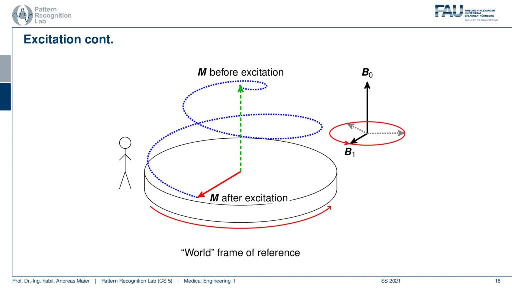
Then we kind of bring our M from the alignment with the main magnetic field and we kind of tip it in the circling motion onto our excited state where it will then continue to circle around the main magnetic field. Now, this is kind of difficult because we have a 3D coordinate system and we have this complex motion if we observe it from the outside. So you can think of this as a world frame of reference and there is essentially this rotating platform that is aligned with the main magnetic field. This motion is very complex to describe. It’s much easier to describe this coordinate system if you step onto the platform.
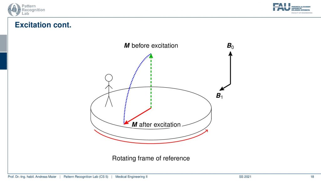
If you were located on the platform so you just step on the platform then you would see that the excitation and the actual motion can be described much easier. So here now we only have the effect that we tip. So if you’re on the rotating coordinate frame the rotating reference frame then it will just be a tipping and the entire motion in this direction will be all gone. We have a much simpler system to describe all of those effects. So this is now why we only stick to two directions. We take the orthogonal direction and the direction along with the main magnetic field and then we can describe the effects much easier.
So this then brings us to the problems of relaxation and contrast.
We’ve already seen that we’re able to generate different contrasts and this is related to the relaxation properties. In contrast to the excitation where we just essentially flip our switch, the difference is that now we have a difference in relaxation. So the relaxation in the two different directions is different. We have a relaxation and the main magnetic field direction and the relaxation in the perpendicular one. You’ll see that in the orthogonal direction the magnetic field is diminished much quicker than it actually takes to return to the main magnetic field direction. So this is caused because of the neighboring hydrogen nuclei. So they also influence each other you remember there’s many of them and this means that they influence each other. This is the reason why in the transverse direction we have the magnetization removed much quicker because all of these hydrogen atoms they’re actually interacting with each other. So what we actually observe in terms of magnetization is not the magnetization of a single hydrogen nucleus. But we are measuring essentially the average over the entire voxel. Of course, because a single nucleus would be way too small to be actually measured. So we essentially measure the average effect and this gives rise now to the two different relaxation times.
So what we get is essentially a voxel-based resolution. Here you see now that we kind of get the relaxation over the virtual 3D units that we need to introduce to reconstruct the images and all that we are getting is essentially the mean over the entire voxel.
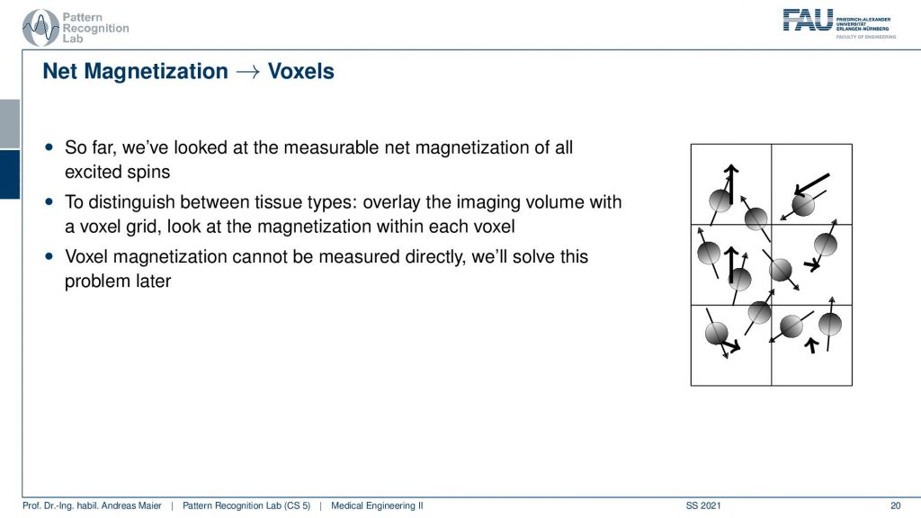
So then this is embedded in a voxel grid and the voxel grid is then the actual property that we want to reconstruct. So right now we won’t care about how to actually resolve the voxels. So this will actually be the topic of the next video so we won’t talk about that. But we are only interested in the properties of let’s say one big voxel that’s all we’re measuring right now one big voxel and in the next video we will see how we can partition the big box into smaller units.
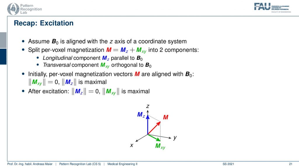
So what we’ve seen is that we have the excitation which just pushes on the switch and now we’re color-coding this here. We differentiate the two directions the B0 field we define now in this context to be aligned with the z-axis of the coordinate system. Then we can essentially compute a split per voxel into the magnetization M which is the total magnetization that is the magnetization in the z-direction plus into the x, y-direction. So this is the longitudinal component Mz which is parallel to the B0 and then we have the transversal component which is orthogonal to B0. So this is a very important element that we have to distinguish in order to understand the following effects. Now if they are aligned completely with B0 then we have a maximum magnetization in that direction and the transverse direction is exactly zero. After the excitation in the ideal case, we have an excitation that completely flips and then we have an excitation that is completely in the transverse direction and zero in the longitudinal direction. So this is the state then after excitation.
Now what happens is that we have two types of relaxation. So we have two processes and they are not entirely independent because we have the neighboring voxels. This means that we have interaction between the hydrogen nuclei in particular in the transverse direction. So the recovery of the longitudinal component is much slower than the decay of the transversal component in xy-direction. This happens on two different time scales and this is the key element that will enable us to get different contrasts and we’ll see that on the next line.
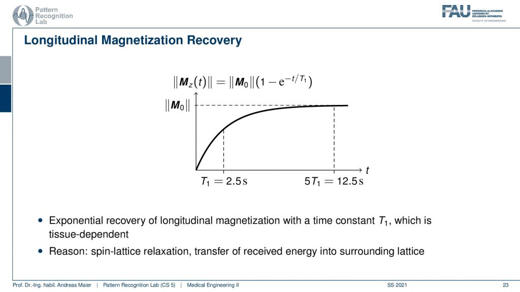
So the longitudinal recovery so going from zero to the maximum magnetization along the direction of B0 you see here. It takes about you could say the time to double is about 2.5 seconds here in this example and after 5 T1 it is in the range of 12.5 seconds. So in order to completely recover and have the alignment, it takes 12.5 seconds.
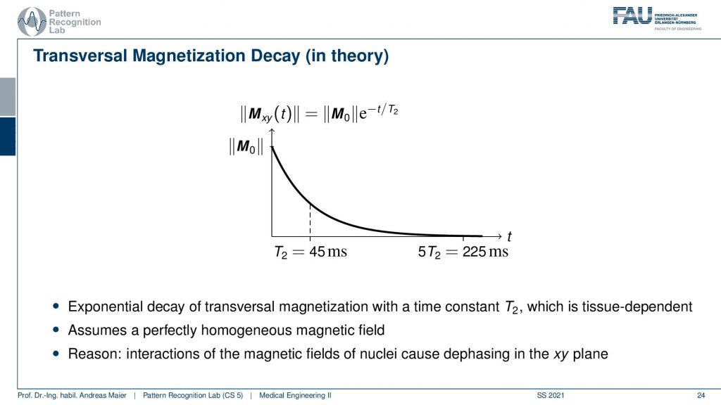
Now the decay in the other direction is much quicker. So this is the so-called T2. This is the loss in the transverse direction and this has a time to half itself of approximately 45 milliseconds. If you now wait for 5 T2 then you’re in the range of 225 milliseconds. So this happens at a much much higher rate. So you very quickly have the decay going on and then it takes a long time until the T1is kicking in and you get essentially the recovery and the longitudinal direction. This gives rise to two different contrasts and the two directions.
Now what you also have to keep in mind is that there are additional effects, not just the neighboring voxels but also the B0 the main magnetic field is actually never perfectly homogeneous. Because of that, there is additional interference between the decay and that actually causes the so-called dephasing to happen much quicker than the actual T2. If you measure that time that’s actually the T2* star which is always smaller than the T2 time and it’s associated with the inhomogeneity in the main magnetic fields.
Now how can we think about this process? Now let’s take our rotating platform here again and now in contrast to the flipping where everything was essentially running on the surface of the sphere, we can now see that the relaxation in the magnetic field main direction takes much longer than the decay in the orthogonal direction. So we observe what you can see here on this figure. Now, this is a kind of difficult motion. Let’s step onto the platform again and you can see now that instead of running on a circle we first have to decay in the orthogonal direction and then we slowly build up in the parallel direction. So this is a typical curve and this curve is essentially driven by tissue parameters. So if we know T1 and T2 this is also a characteristic of the material that is predominantly present in the voxel. This can also be used to figure out what kind of material is actually in that voxel. So it’s not just contrast but we can also figure out some effects of that material.

If we now want to image we need a protocol and what happens is typical that you have the impulse.
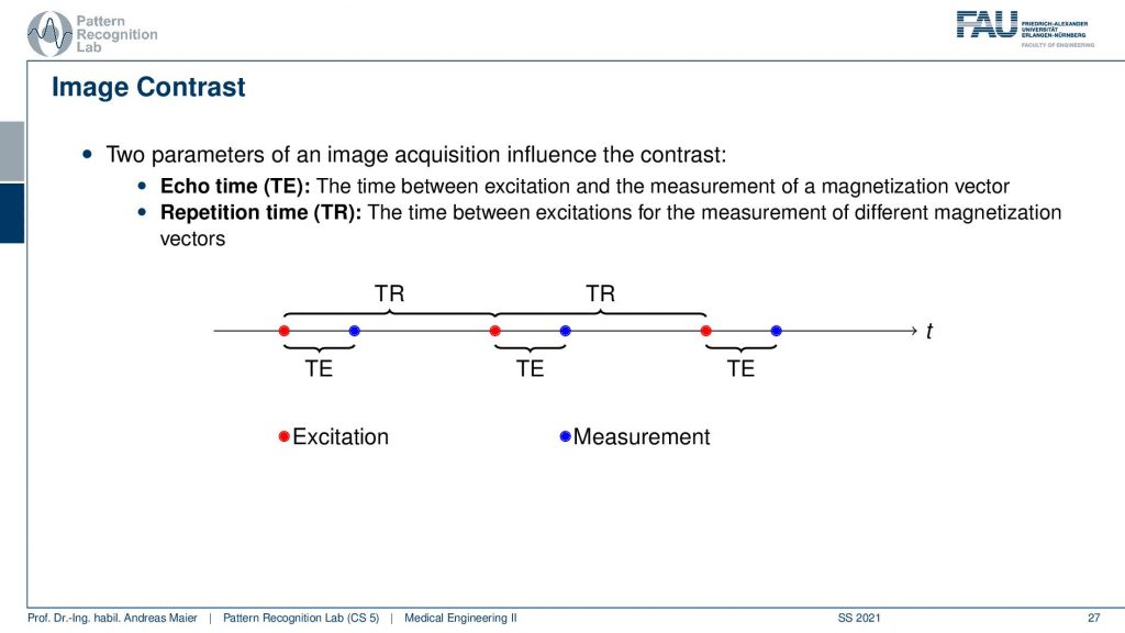
So you play the pulse and then you take some time for the excitation. So this is the TE and after the excitation time, you can then actually start reading out. Then you wait some time this is the repetition time, the TR and then you play the next pulse. So we have the excitation, the time until we have the readout that’s the TE and the TR is the time until we repeat the next pulse. So if we use those two different concepts we can now use them to figure out the T1 and the T2 times.
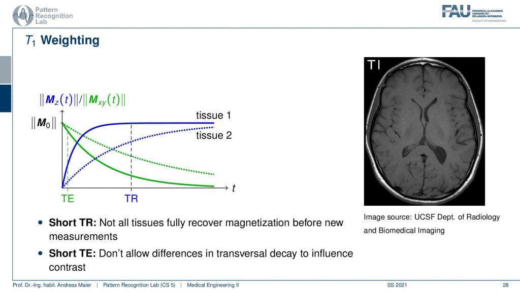
This leads us then to T1, T2, and other weightings. Now in a T1 weighted sequence, you try to figure out the properties of the T1 time. So you have a short repetition time and you also have a short readout time. Now if you look closely at this plot you can see that the short echo time actually prevents the two signals to have large differences in T2. So you pick them very short such that the actual difference between the two different tissues here in T2 doesn’t play a role. Then you also pick a short repetition time such that the two tissues have barely time to recover in terms of T1. So if you do that repeatedly over a series of pulses you will see that then this difference here in T1 will make the main contrast while the difference here in T2 is not able to emerge.
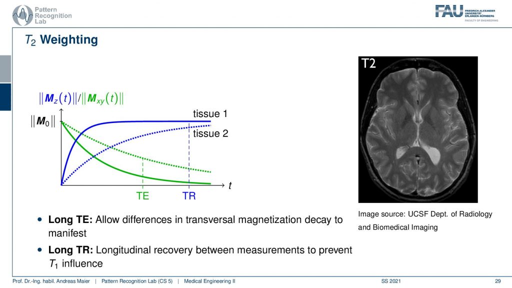
Now if you do that with a different setting and you have a much longer echo time. So you wait before you actually read out then you have this strong difference in T2. Then you also wait very long for the repetition time such that the difference in T1 is almost gone and this will be able to measure a T2 weighted sequence. So if you have a long repetition time and a long echo time you get a T2 waiting. If you have a short repetition time and a short echo time you get a T1 weighting.
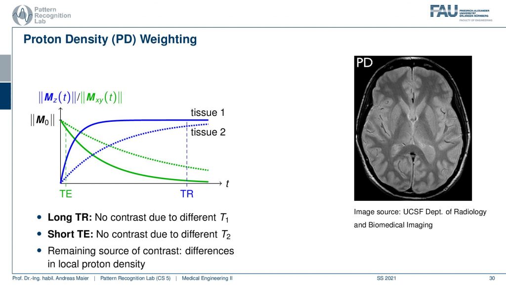
Now you can of course also explore the other configurations. One particular one that you could think of is a short echo time such that there is almost no difference in the T2 time and also a long repetition time such that there is almost no difference in the T1 time. So this way you get something that is essentially only weighted with the number of protons and this is then called the proton density mapping or proton density weighting. With these kinds of maps, you kind of gets the number of hydrogen nuclei per voxel. You could also be thinking about the exact opposite.
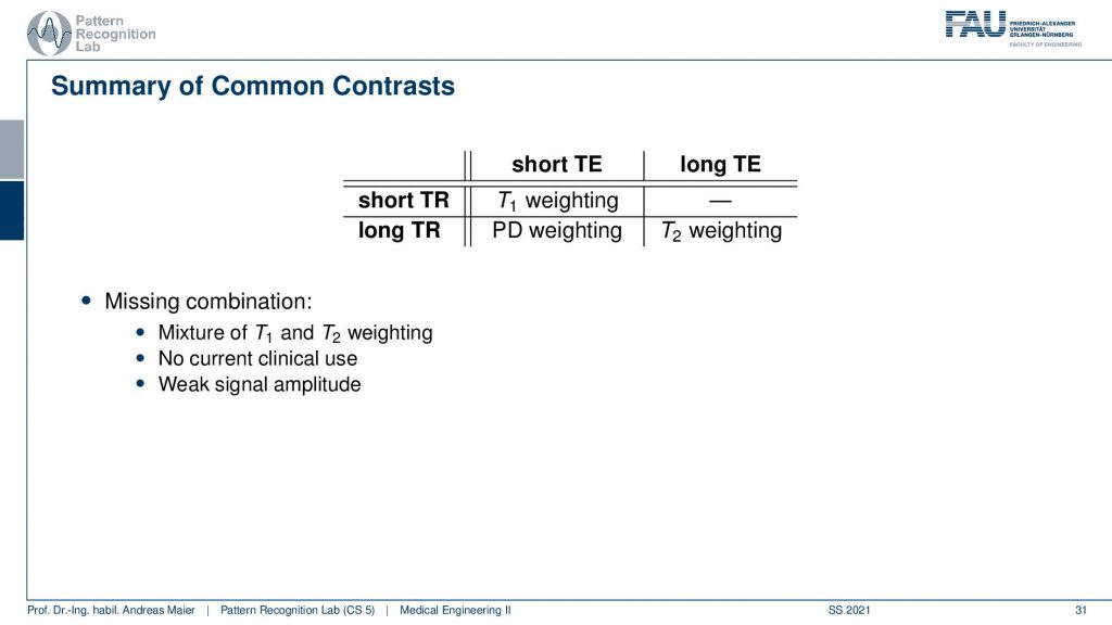
So you could also have a short repetition time and a long echo time but this is a combination that you essentially never find in practice. Because it just generates a very big signal amplitude. So these are the main contrasts that are being used in MR imaging and now you have seen how the resonance effect can actually be generated and how the difference in the relaxation can be used in order to get different image contrasts.
So this already brings us to the end of this video. So you’ve seen now all the basics of magnetic resonance. So you’ve seen the resonance effect. We introduced it with the very simple example of a compass needle and then we went on in that we have a magnetic field that has to be repeated which then gave rise to using an rf coil in order to get this varying magnetic resonance effect. So this way we can then excite the small compass needles in the body. Once we excited them we can actually record the echo effect and if we do that in different configurations we can then play with the echo time and the repetition time in order to figure out the T1 and the T2 factors that are the difference between the decay in the transverse direction and the growth of the signal in the parallel direction. So these are the two main effects that we can use for imaging. We’ve seen that from different combinations of TE and TR we can build then three different types of contrast. To be honest, there is much more MR contrast because it’s not just the T1 and T2 factors and the relaxation and transverse and parallel direction but it’s also that you actually have the other effects. You’ve seen the dampening fluid and so on. Also, the bindings of the molecules of the different atoms have effects on the relaxation and they can also be used in order to determine particular contrasts but we’ll not discuss in detail how to measure those contrasts. Yet there is some more that we have to talk about. Right now we essentially just measured a single huge voxel and measured the T1 and T2 kind of relaxation inside of that voxel. Now we want to go ahead in the next video and really resolve the voxels into the different spatial orientations. You’ll see that a good old friend of ours will pop up again and you will be quite surprised that a very typical transform that you already heard about in our chapter on signals and systems is coming back. So thank you very much for watching this video and looking forward to seeing you in the next one, bye-bye.
If you liked this post, you can find more essays here, more educational material on Machine Learning here, or have a look at our Deep Learning Lecture. I would also appreciate a follow on YouTube, Twitter, Facebook, or LinkedIn in case you want to be informed about more essays, videos, and research in the future. This article is released under the Creative Commons 4.0 Attribution License and can be reprinted and modified if referenced. If you are interested in generating transcripts from video lectures try AutoBlog
References
Maier, A., Steidl, S., Christlein, V., Hornegger, J. Medical Imaging Systems – An Introductory Guide, Springer, Cham, 2018, ISBN 978-3-319-96520-8, Open Access at Springer Link
Video References
- How dangerous are magnetic items near an MRI magnet? https://youtu.be/6BBx8BwLhqg
- MRI Cryostat Vacuum Lost https://youtu.be/CXWqIz68eqw
- MIT Phyics Demio – Bicycle Wheel https://youtu.be/8H98BgRzpOM
- NMR Spectroscopy Visualized https://youtu.be/RZLew6Ff-JE
- Uri Geller https://youtu.be/pN_AC9KHlM8
- Randy Dickerson – Syngo Via VB20 Cinematic Rendering https://youtu.be/I12PMiX5h3E