Lecture Notes in Pattern Recognition: Episode 20 – Multi-layer Perceptron

These are the lecture notes for FAU’s YouTube Lecture “Pattern Recognition“. This is a full transcript of the lecture video & matching slides. We hope, you enjoy this as much as the videos. Of course, this transcript was created with deep learning techniques largely automatically and only minor manual modifications were performed. Try it yourself! If you spot mistakes, please let us know!
Welcome everybody to pattern recognition! Today we want to look into multi-layer perceptrons that are also called neural networks. We’ll give a brief sketch of the ideas of neural networks.
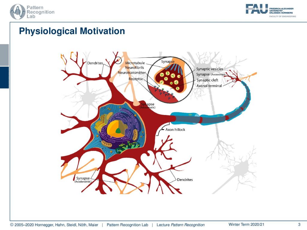
Let’s have a look at multi-layer perceptrons. You see that we talked about this here only about very basic concepts. If you’re interested in neural networks we have an entire class on deep learning where we talk about all the details. Here we will stay rather on the surface. You may know that neural networks are extremely popular because they also have this physiological motivation. We’ve seen that the perceptron is essentially computing a sum of elements that go in, they are weighted in an inner product and some bias. You could say that this has some relation to neurons because neurons are connected with accents to other neurons and they are essentially getting the electrical activations from those other neurons. They are collecting them and once the inputs are greater than a certain threshold then the neuron is activated. And you typically have this zero or, one response. So, it’s either activated or not and it doesn’t matter how strong the actual actuation is. If you are above the threshold then you have an output and if you’re not there’s simply no output. If you are interested in the biology of learning and memory, please see this excellent introduction by Prof. Schulze.
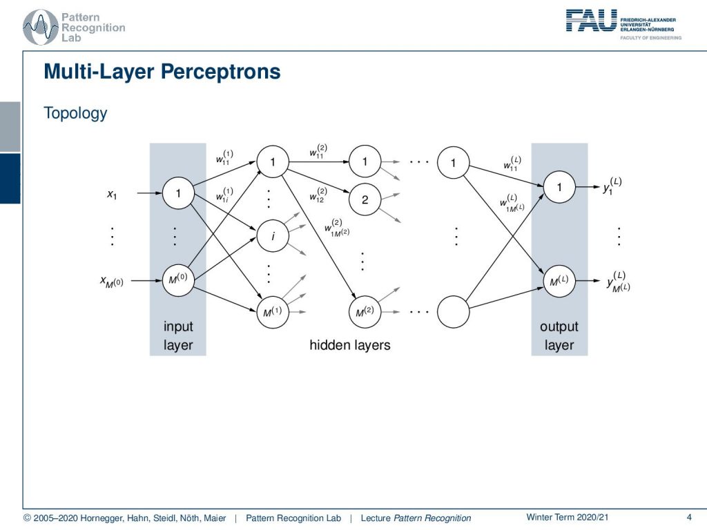
Now, you have these neurons and we don’t talk about biological ones here. But we will talk about the mathematical ones based on the perceptron. Then we can go ahead and arrange them in layers and layers on top of each other. We essentially have some input neurons where we simply have the input feature vector and some bias that we’re here indicating with one. This is then passed in a fully connected approach. So we are essentially connecting everything with everything and we have then hidden layers. They’re hidden because we somehow cannot observe what is really happening with them. We can only observe that if we have a given input sample and we know the weights then we can actually compute what is happening there. If we don’t have that then generally we don’t see what is happening but we only see the output at the very end. The output then is observable again and we have typically the desired output. This desired output can then actually be used to compare this to the output of the network, which allows us then to construct a training procedure. Note that we are not only doing sums of the input elements that are weighted but what’s also very important is this non-linearity.
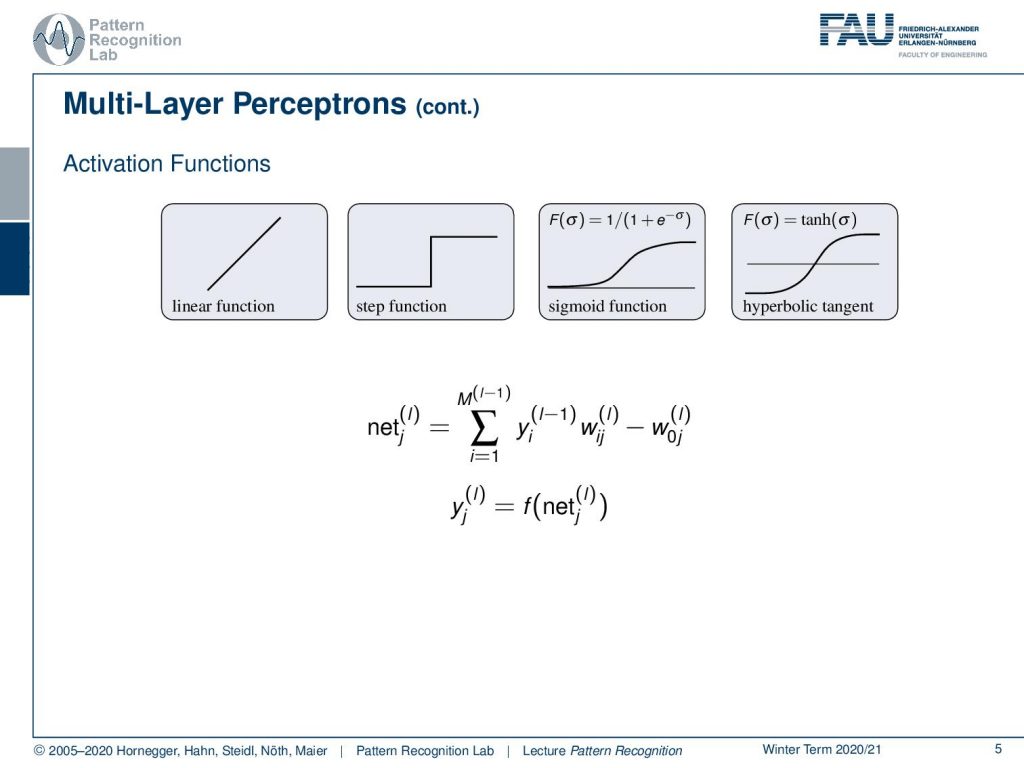
So we kind of need to model this all or none response function. We’ve seen that Rosenblatt originally was using the step function. Of course, we could also use linear functions but if we were using linear functions we will see that towards the end of this video then everything would essentially collapse down to single big matrix multiplication. So, actually in every layer, if they are fully connected then you’re essentially computing a matrix multiplication of the activations of the previous layer with the next one. This can be modeled simply as a matrix. Now, what is not modeled typically as a matrix is the activation function and the activation function is applied element-wise. The step function was this approach as Rosenblatt did it. But in later approaches and classical approaches, the following two functions the sigmoid function and the logistic function were very commonly used and as an alternative also the hyperbolic tangent was used because it has some advantages with respect to the optimization. So, we can now write down our units of these networks as essentially sums over the previous layers. So we have some yi that is the output of the previous layer. So we indicate this here with L minus 1. This is then multiplied with some Wij and we also have this bias W0j in the current layer L. This sum is essentially constructing the output already but the net output is then also run through the activation function f and f is one of the choices that we see above here. So, this is introducing the non-linearity that is then producing the output of the layer L in the respective neuron.
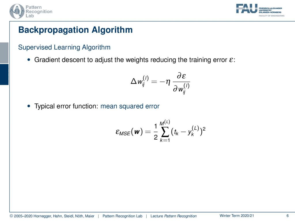
Now, you want to be able to train this and this is typically done using the backpropagation algorithm. This is a supervised learning procedure and backpropagation helps you to compute the gradients. So backpropagation is actually not the learning algorithm itself, but it’s the way of computing the gradient. Here, we propose to use gradient descent and we can essentially do that by then updating the previous weights following the gradient of the weights. We can then essentially determine this by a partial derivative of a loss function here denoted as ϵ and this is then partially derived with respect to all of the weights of that particular layer. You can see if you think in layers you will find that all the weights of the respective layer get very similar update rules. Therefore they can be summarized and we will do that in the following couple of slides. So typically you choose an error function here we choose the mean squared error. There are many other loss functions also available if you want to see all the details about other common loss functions I can really recommend to look at the lecture on deep learning. Here you see we have some target tk and then we compare the output of the last layer and take the square of that and sum up essentially this for all of the outputs. This gives us the mean square error.
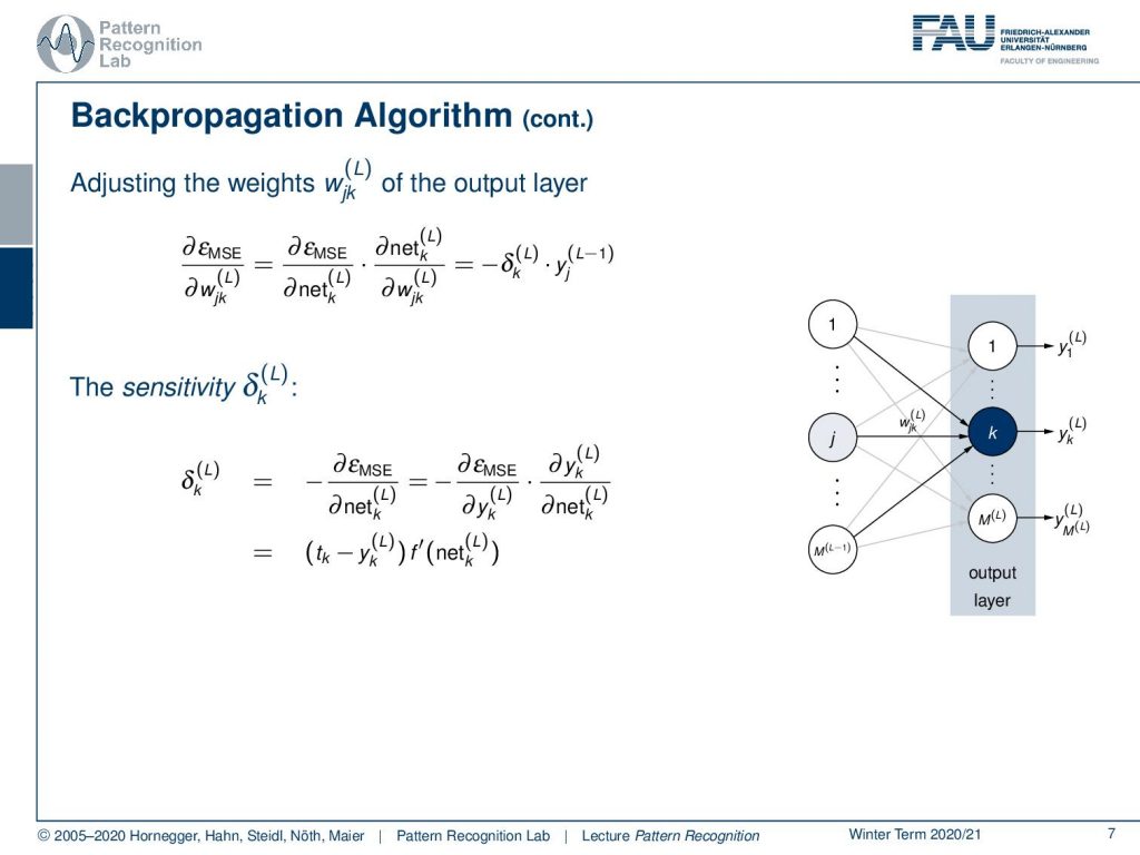
Now how can we compute the updates? Well, we need to compute the partial derivatives with respect to the weights that we want to update. We will start with the output layer so here you essentially have the mean square error. We then compute the partial derivative with respect to the actual last layer weights. If we want to do that we see we have to apply the chain rule. So we’re computing the partial derivative of the error with respect to the net. Then the partial derivative of the net with respect to the weight that we want to update. If we look at this in more data we can already see that the partial derivative of the net with respect to the weights is simply the output of the previous layer. So, this is the yj of layer L minus 1 which is essentially the layer before the last layer. Then we introduce this δk(L), which is essentially the so-called sensitivity. Now the sensitivity we can look at in a little bit more detail. Here we need to compute the partial derivative of the error with respect to the net and again if we want to look at that we can apply the chain rule. So we compute the partial derivative of the error with respect to the last layer output. Then the last layer output we compute the partial derivative with respect to the net in that layer. Then you can see that we can essentially write this up as the target value minus the last layer output times and now we have f prime here that you know it’s the derivative of the activation function of the net at the layer L. So this gives us the sensitivity in the last layer.
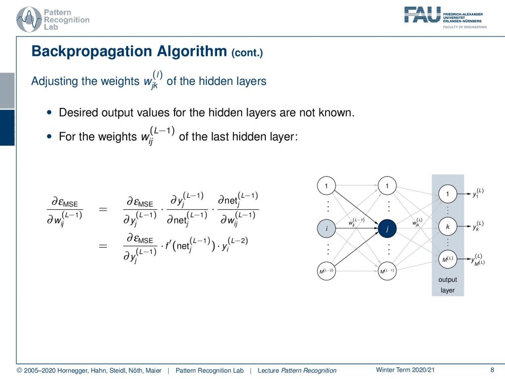
This was fairly easy. Now let’s look at what happens if we go one layer deeper. So we want to go now for the weight of the l minus one layer, the last hidden layer. If we want to do that we essentially follow the same line and we take the mean square error and compute the partial derivative with respect to the weight of the last hidden layer. Now we can see that we apply again the chain rule. So, we compute the partial derivative of the mean square error with respect to the last hidden layer outputs. Then we can see that we need to compute the partial derivative of the last hidden layer outputs with respect to the net and again the net with respect to the weights. Well computing the partial derivative of the net with respect to the weights will simply give us the input from the previous layer. So this is simply yi of the previous layer. So this is L minus 2. Then again computing the partial derivative of the L minus 1 layer output with respect to the net is going to give us the derivative of the activation function of the net. We still have to compute now the partial derivative of the mean square error with respect to the output of the L-1 layer.
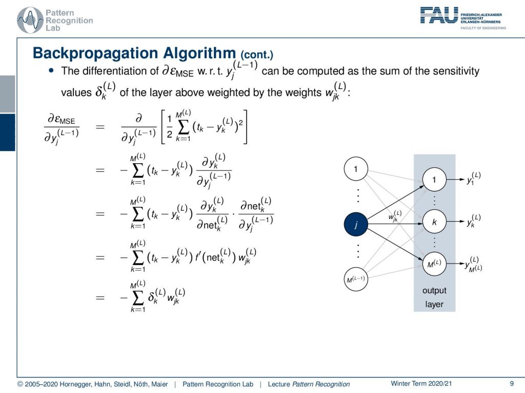
So, we can see now that this partial derivative of the mean square error with respect to the L minus 1 layer is a little bit more complex. Because the mean square error is essentially the difference between all the outputs and compared to the targets of the power of two and summed up. So in order to compute the next step, we apply again the chain rule. So we are computing the partial derivative with respect to the square and we see this gives the first term. So this is the sum over all of the activations in the last layer compared to the target values. Then we still have to multiply this with the partial derivative of yk of the layer L with respect to the yj of the layer L minus 1. Now again we apply the chain rule here so this then gives us the partial derivative of yk of layer L with respect to the net of layer L. Then we still get the partial derivative of the net at layer L with respect to the inputs that are created in the L minus 1 layer in yj. Now we can again see that we can determine these partial derivatives. This is again the partial derivative of the activation at the position of the net at layer L. This is multiplied then with the next partial derivative and again the net with respect to the previous layer is simply the weights. So if we write this up again as sensitivities you can see that we essentially have the sum over all the sensitivity is multiplied with the respective weights that we get here as the mean square error backpropagated to the L minus 1 layer.
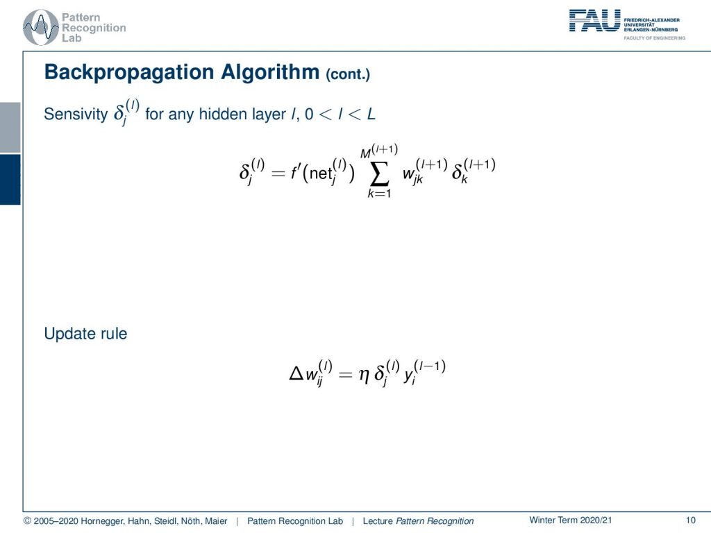
Now, we can use this term again and compute the final gradient update and here we see then that we get for the sensitivity in any layer L. It is simply the derivative of the activation function of the net times the sum over all the weights multiplied with the sensitivities of the next layer. So, we can essentially then formulate this as a kind of update rule. The update rule, if we want to create the gradient of the weights, is then given as the sensitivities of that layer times the input of the previous layer. So we kind of get this recursive formulation to compute those updates. Now, this is looking at all of the weights on the node level, and looking at this on node level is extremely tedious. I think this is a bit hard to follow this is why I also brought to you the layer abstraction concept.
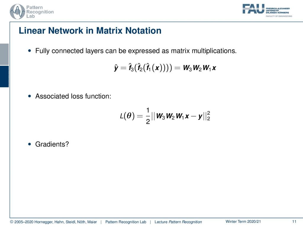
In the layer abstraction concept, we now simply express the different layers as matrix multiplications. Here in this academic example, I’m also skipping over the activation function. So, if you want to include the activation functions then you also need to apply them element-wise after each application of the matrix multiplication here. Then this would really give you a full net. Here we essentially have three matrices multiplied to each other, technically they could also be collapsed to a single matrix but in order to show you the workflow of the derivations, I will use this example. So if you do that and go ahead then we also need our mean square error, this is now simply the L2 norm squared of the desired output and the respective input parsed by the network. So this is essentially then x times W1times W2 times W3 minus the desired output that we denote here is y. So, this is essentially exactly this mean square error. Note that I’m mixing a bit the notation, but of course, this is an advanced class and I think you can now understand that the y is no longer the output of the net, but here it is the desired target. So, if we now go ahead we need to compute the gradients and I’m not going through this example and really compute all of the gradients. But what I want to show you is the general sketch of how the back-propagation is then actually applied.
So, if you want to compute the gradients then the first thing that you do is compute the forward pass through the entire network. Then you need to compute the updates with respect to the different layers. So of this loss function here you compute the partial derivative of the loss function with respect to W3, W2, and W1. Now W3 is the last layer. So what you get in terms of the update for W3 is the partial derivative of the loss function with respect to f3 of x so this is essentially the output of the net. Then you multiply this with the partial derivative of f3 with respect to W3 and I’m writing the actual computations down here so that you can actually follow this gradient. Now if I go back one layer then I’m essentially reusing the result of the previous layer partially, because if I want to back-propagate for another step then I essentially need for each of those layers the partial derivative with respect to the inputs and the partial derivative with respect to the weights. So in the W2 layer, this is then going to be the partial derivative of f3 with respect to f2. And this is simply going to be W3 transpose and then you also need the partial derivative of f2 with respect to W2which is then the input from the previous layer transposed. Now if I want to compute the complete gradient I’m essentially multiplying the partial derivatives following this red path here. Then I get the gradient update for that particular weight. So the deeper I go, the more often I have to multiply with the partial derivatives that are needed to back-propagate to that particular position. If I want to go to the very first layer you see that I have in total four multiplicative steps in order to compute the update for the first We have more of this example in the deep learning lecture. So there we go into more detail also about back-propagation and how to compute the individual steps. But I think this figure here and the node-wise computation is sufficient at this point.
You see now that we actually have a physiological background for neural networks. We didn’t talk about the details about the neurons the synapses and the action potentials. But I will give you references if you’re interested in the biological background. This then gave rise to a topology of multilayer perceptrons that we arrange in layers. Of course, in every layer, we apply neuron wise activation functions. If we then want to compute updates we can use the back-propagation algorithm in order to compute the actual gradients. Then we can try gradient descent methods in order to actually perform the training.

So, in the next video, we want to talk a bit about optimization strategies in more detail. We will look into some ideas on how we can perform optimization and I still have some further reading for you.
In particular, if you’re interested in physiology I can recommend these two references. They are all very nice if you want to get some understanding of the actual biology that is associated with biological neural networks. So I hope you liked this small video and I’m looking forward to seeing you in the next video. Thank you very much for watching and bye-bye!
If you liked this post, you can find more essays here, more educational material on Machine Learning here, or have a look at our Deep Learning Lecture. I would also appreciate a follow on YouTube, Twitter, Facebook, or LinkedIn in case you want to be informed about more essays, videos, and research in the future. This article is released under the Creative Commons 4.0 Attribution License and can be reprinted and modified if referenced. If you are interested in generating transcripts from video lectures try AutoBlog
References
- Robert F. Schmidt (Hrsg.): Neuro- und Sinnesphysiologie, 3., korrigierte Auflage, Springer, Berlin, 1998
- Robert F. Schmidt, Florian Lang, Martin Heckmann (Hrsg.): Physiologie des Menschen mit Pathophysiologie, 31., neu bearb. u. aktual. Auflage, Springer, Berlin, 2010