
These are the lecture notes for FAU’s YouTube Lecture “Pattern Recognition“. This is a full transcript of the lecture video & matching slides. We hope, you enjoy this as much as the videos. Of course, this transcript was created with deep learning techniques largely automatically and only minor manual modifications were performed. Try it yourself! If you spot mistakes, please let us know!
Welcome back to pattern recognition. Today we want to start talking a little bit about optimization and we’ll have a couple of refresher elements in case you don’t know that much about different ideas and optimization. You will see that they’re actually fairly simple and they will turn out to be quite useful for your further work and pattern recognition.
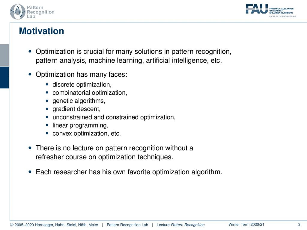
So today’s topic is optimization and of course, this is crucial for many things in pattern recognition. So you want to find solutions to complex objective functions and this is a problem that arises in pattern analysis, machine learning, artificial intelligence, and the like. So, optimization also has many phases. There’s discrete optimization, there’s combinatorial optimization genetic algorithms gradient descent unconstrained and constrained optimization linear programming and convex optimization, and so on. So here we essentially need some basic knowledge on optimization such that you are able to follow the remaining lecture. This is why we want to talk about a couple of ideas on how to optimize and of course, everybody has typically his or her own favorite algorithm. Therefore we will show some of the ideas and in particular, what we will focus on in this class is the optimization of problems that are convex.
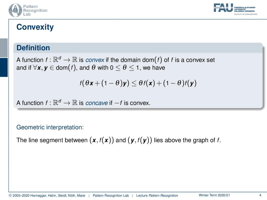
So here you see the formal definition of convexity. A function probably a high dimensional one of dimension d that is projected onto a scalar value is convex if the domain of f is a convex set and if for all points x, y within this domain and θ between 0 and 1 we have the following relation. Here you can see that we have f(θx + (1 – θ)y). So you can essentially see this is a linear interpolation between x and y. So if you’re moving in the input space from x to y then all of the points on the function will fulfill the property that if you interpolate linearly between f(x) and f(y). So here we use the same notation. So, it’s θf(x) + (1- θ)f(y). So this is again a linear interpolation in the output domain and this will always be greater than the interpolation along the original function. So you can also see that a function is concave if -f is convex. If we look at this in a kind of geometric interpretation, we can say that the line segment that lies on (x,f(x)) and (y,f(y)) lies above the graph of f. If you can connect any two points on the graph with a line and the slice above the graph of f, you have a convex function. A very typical example is a parabola.
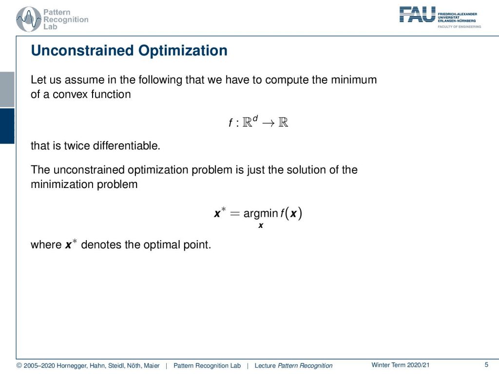
Let’s look a bit into unconstrained optimization. So here we generally assume that we have some function from R^d to R that is twice differentiable. Now the unconstrained problem is just the solution of the minimization problem x* equals to the minimum over f(x) and here x* is the optimal point.
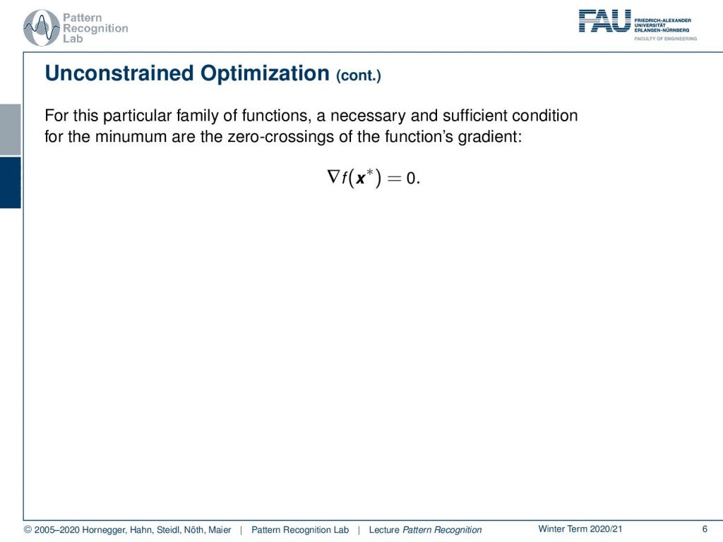
If we have this particular set of functions meaning convex functions a necessary and sufficient condition for the minimum are the zero crossings of the function’s gradient. So if you have a convex function and you find a position where f(x*) and the gradient at this position is zero, then you must have a minimum. The great thing is that if you have a convex function and you seek to find the minimum then following the negative gradient direction will eventually bring you there. So, this is already a very nice thing, and also by the way you will find a global minimum in a convex function. So the convex function has only one global minimum. The gradient descent methods here will always result in global minima, which is also very nice in terms of optimization. Because that essentially means you are not really dependent on the initialization. It doesn’t matter where you start the gradients will always lead you to the global minimum.
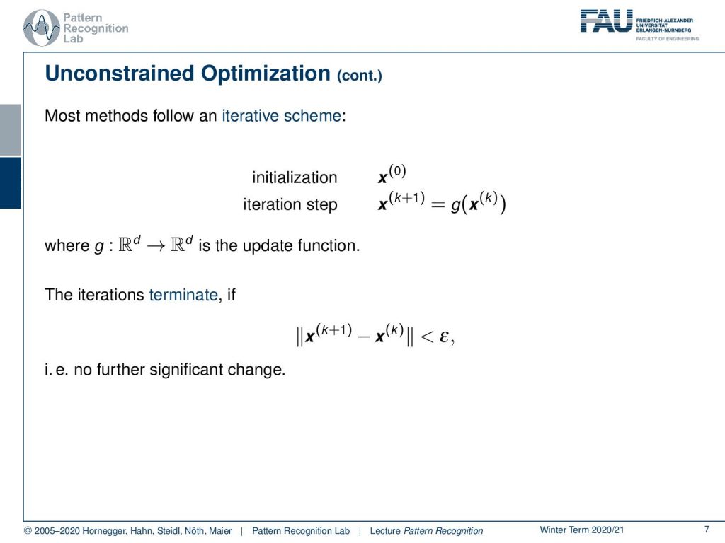
Now, most methods in this unconstrained optimization follow this iterative scheme. You initialize somewhere with some x(0) that you can choose randomly essentially or, you have a fixed value. Then you do iteration steps and you produce a new x(k+1) of the old x(k) given some function g and g is the update function. So, there are different versions of implementing g, one could be just following the negative gradient direction. Another one could be shrinkage functions. So these are functions that allow you to produce a smaller function value for a given input of x. Now the iterations terminate if we only have a small change meaning that the difference between x(k+1) and x(k) is small below a threshold that we introduce here as ϵ. So there is no further significant change.
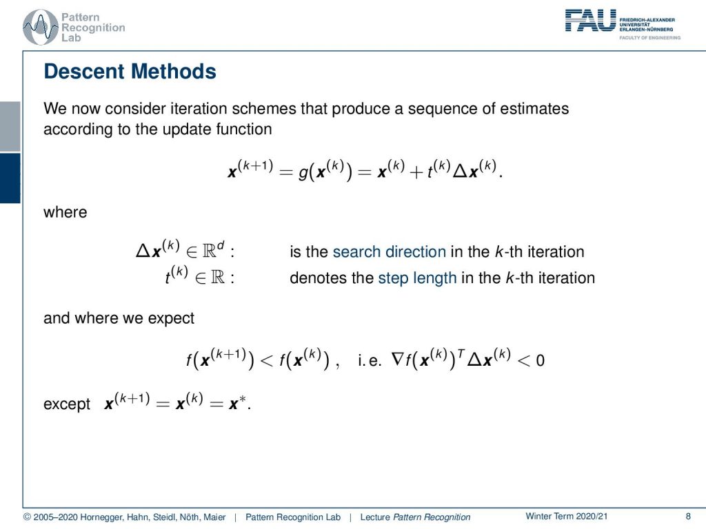
Now let’s consider a very simple update scheme I already hinted at that. We choose the update function to be the old position plus some step size t(k) times ∆x(k) and here ∆x(k) is the surge direction in the cave iteration and t(k) denotes the step length in the current iteration. Now we would expect that if we find a better position for x(k+1) then of course the function value of f(x(k+1)) will be lower than the function value of f(x(k)) and there is also the inner product of the gradient with our update direction should be negative. So, this should be a value that is below zero. Of course, this will be generally the case unless we have x(k+1) equals to x(k)equals to the optimum x*.
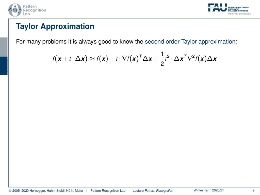
Also, one thing that you want to keep in mind for many problems: it’s always good to know the second-order Taylor approximation. Here we introduce the Taylor approximation for our twice differentiable function. So, you can see that I can approximate f(x+ t ∆x) can be approximated as f(x) plus t times the gradient of x inner product with the step direction the update direction ∆x plus 0.5 t squared times the inner product of our update direction with the hessian times the update direction. So, this is an approximation of the actual step size in this direction. This is also very commonly used in second-order methods.
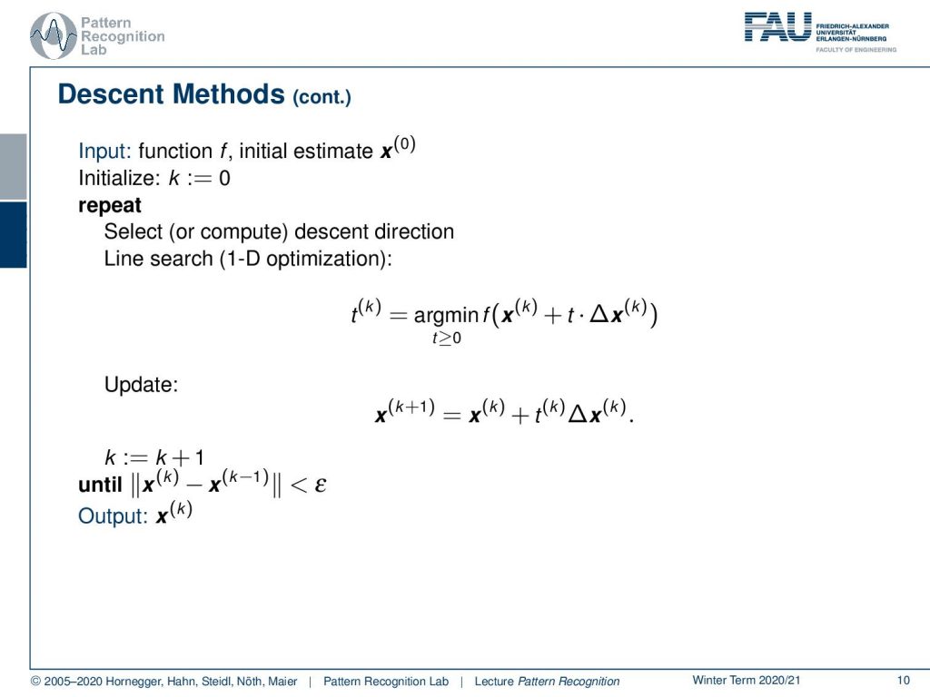
Now let’s start with some simpler idea. We want to talk about descent methods and here we want to have an initial estimate x(0) and we have some function f. Then we initialize with k equals to 0. Now, we select or compute the descent direction. In a simple case, we can just take the negative gradient direction, but we will see there are also more sophisticated ways of choosing this. This is why we have this general form using this ∆x. Then we do a line search which is essentially a 1D optimization and there we choose essentially the optimal step size t. So we determine t(k) as the minimum over f(x(k))plus t times ∆ x(k). So, this will allow us to get the minimum in the search direction. Then we update accordingly with the optimal step size t(k) times ∆x and we add that to our old position x(k). Then, we increase our iteration counter and we do repeat this until we only have a very small difference between the previous and the new iteration, below some threshold ϵ. We can then return our x(K).
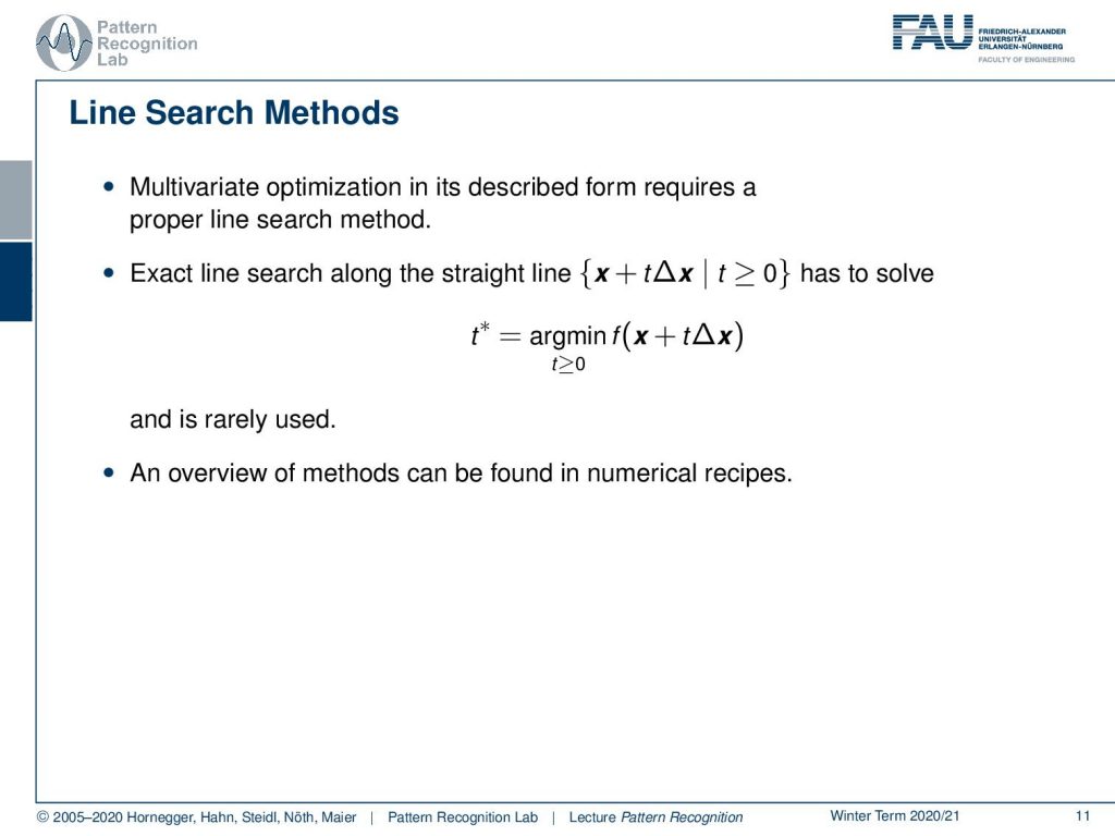
Now let’s talk a bit about the line search. The line search is typically conducted in multivariate optimization where you have a high dimensional problem where you want to work on. Then you need a proper search method. So one thing that you could do is of course an exact line search where you then try to solve essentially really this minimization problem. It’s only a one-dimensional problem. But probably it would involve many accesses to the actual function value. So you would have to really try to find the minimum for t and therefore this is rarely used. There’s a couple of different choices for this line search method and there’s a very good book called Numerical Recipes. If you look into Numerical Recipes by the way it also comes with implementation. So it also has code examples and so on. So Numerical Recipes is a really good book if you want to get into the coding of optimization and it’s available in different programming languages. So let’s look into the simple idea of having a fixed step size.
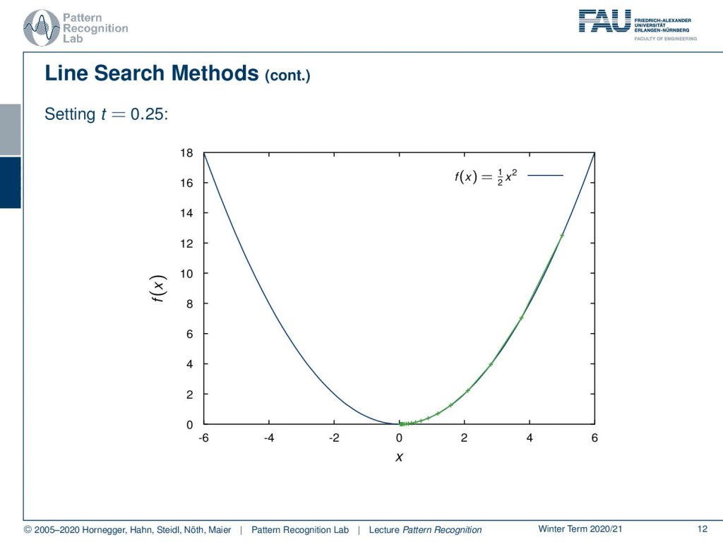
If you do that and here we choose our step size as 0.25, then you can see we follow the negative gradient direction here and we converge after a couple of steps very nicely to our global minimum of this parabola here. So this works fairly well – but remember – this step size is also dependent on your problem. So you may want to choose different step sizes for different problems.
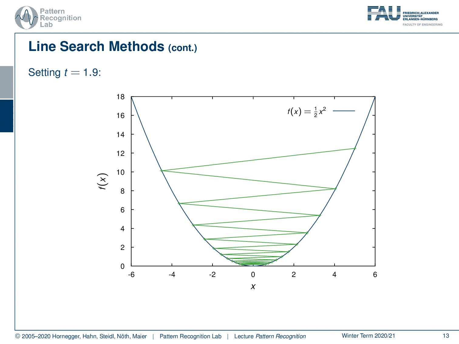
We can show this here: we take the same problem but now we take a step size of 1.9. If you take 1.9, you see we start at the point here on the top right. The first thing that happens is we jump all the way over here. So our step size is too large and then we step back because we follow again the negative gradient direction. This is now showing in the opposite direction which means that we essentially end up on the other side of the parabola again. In the next step, we have to jump back again and so on. You see that our method will eventually converge. But it takes many many many different steps until it really ends up at our desired minimum.
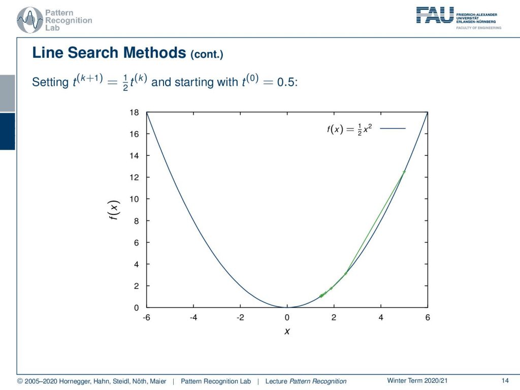
So this is quite an awkward situation. Let’s just reduce the step size during the optimization and here we choose the example that we divide by two in every iteration. We start with an initial step size of 0.5 and here you can see if I do that then we end up not actually at the optimal position but we kind of get stuck on the way towards the minimum. So, also this adaptive step size can have problems. We don’t even reach the global minimum. So this would then also imply a too-small change in x but the reason for the too-small change is not because we actually have arrived at the minimum, but we simply got stuck because we were reducing the step size in every iteration.
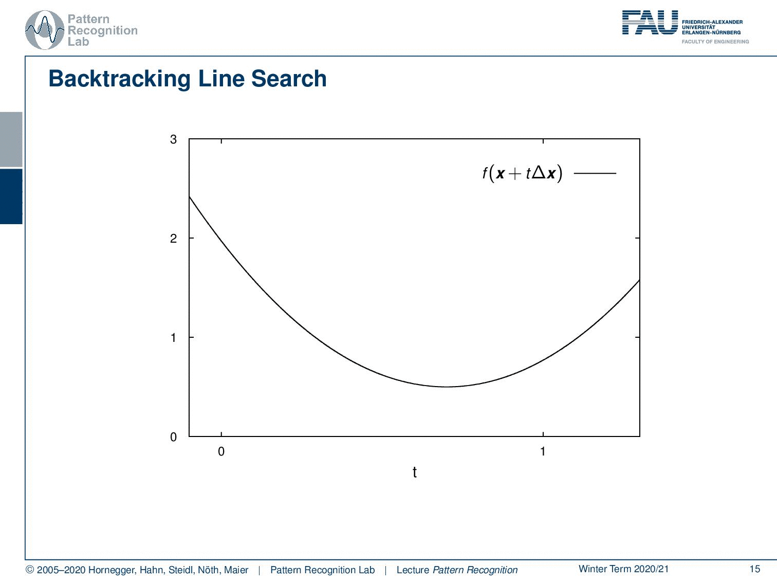
There is an idea that expands on this and this is the so-called backtracking line search. So you see that if we have some position f(x) and this is essentially our parabola where we want to optimize. Then, I can also take the original position f(x) and follow the negative gradient direction. If I would do that I would get this green line here. So this is essentially taking the gradient direction and now I’m projecting this on our step direction which is identical in this case. You see that if I follow this I’m essentially getting a line. Now, this line – because it’s a convex function and I’m following essentially the tangential direction – is always below our graph. Also, note that our inner product of the gradient with our update direction is negative in this case. We are actually having a negative slope because we want to go towards this minimum. So let’s see what we can do. Well one way to approximate this is I could choose some α and I multiply essentially the slope of α and I choose it in a way that we are essentially above our graph. This means that in this case, I have to make this negative value of the slope a little bit smaller. Then I don’t have an as negative slope and you will see that in this case, we find a line that lies at least for a part of our graph above our function. Now if I take this step size α rather large then I may find a point that is even behind the minimum. If we are behind the minimum, in this case, this would then give us the position here. Now you see if I have an appropriate update step, what I’m essentially able to do is I can determine the value of an appropriate update step. So a step size of t that essentially is a good update will produce a function value that is below the line indicated in red here. So as long as I have an update that is probably below the red line, then I probably have found an appropriate update step. So this then allows us to come up with the following update rules.
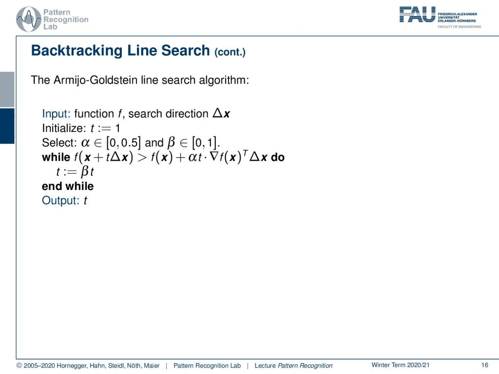
So I initialize with the function and the search direction ∆x. Then I start with a step size of t equals to 1 and I select my α somewhere in the domain between 0 and 0.5. Remember, we have a negative slope so we want this to be a downscaling of the negative slope such that we lie above the graph. We also set some β that is somewhere between zero and one. Now we essentially compute the update position. So we choose the t with one. We take essentially one step for the complete one large t and one large step into this update direction. Then I’m checking whether the position is greater than the red line. So then actually the f(x) plus α times t times the gradient of f(x) inner product with the step direction. If this is the case, this means I’m above the red line then I probably don’t have a very good update. So I do an update of t and there I multiply with β and now β is essentially telling us how to shrink the current step. This is essentially the reason why it’s called backtracking line search because in every update here I’m essentially reducing our step size t until I find a solution that lies below the red line. As soon as I have the position where I’m below the red line then I can output t. Now as a kind of homework, you can think about what happens if we are actually not jumping beyond the actual minimum. You will see then also this line search algorithm will find the solution very quickly. Now let’s put that into some algorithm for updates.
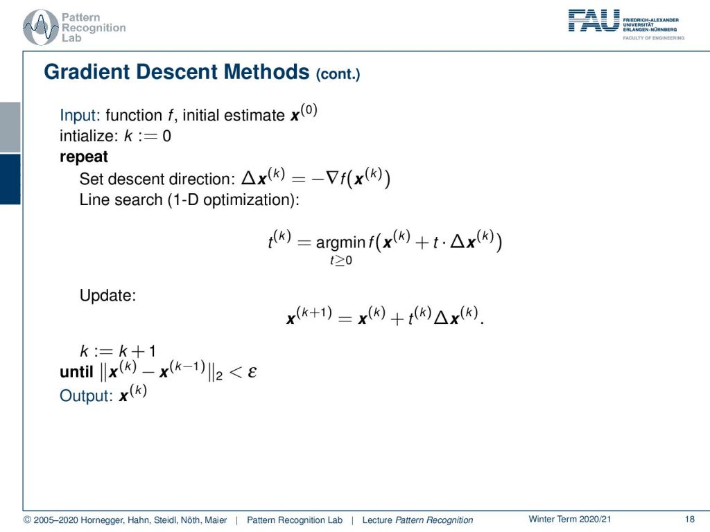
This gives us a gradient descent update algorithm. Here we simply choose the search direction as the negative gradient direction. By the way our rule of thumb is the negative gradient is the steepest descent direction. Now let’s look at this algorithm and you see we start with the function f and an initial estimate x(0). This could be all zeros or a random initialization. Then we start initializing our k equals to zero and we said the descent direction that is here now given as the negative gradient direction. Then we do the 1D optimization, the line search with the for example Armijo-Goldstein Rule and then we can actually compute the update and receive our new position that is now then x(k+1). This is computed from x(k) plus t(k) times ∆x. We increase the iteration counter and we repeat this until we find an appropriate position which means that the difference between the two x’s lies below a certain ϵ. Then we find the output and the output is x(k). So this is the result of our optimization.

Now, this was the first introduction to simple gradient descent methods and line search ideas. We want to continue in the next video and really look into some kind of regularization ideas. How we can combine this with different norms and you will see that this then essentially implies a change in the update direction. So I hope you liked this small video and I’m looking forward to seeing you in the next one. Bye bye!!
If you liked this post, you can find more essays here, more educational material on Machine Learning here, or have a look at our Deep Learning Lecture. I would also appreciate a follow on YouTube, Twitter, Facebook, or LinkedIn in case you want to be informed about more essays, videos, and research in the future. This article is released under the Creative Commons 4.0 Attribution License and can be reprinted and modified if referenced. If you are interested in generating transcripts from video lectures try AutoBlog
References
- S. Boyd, L. Vandenberghe: Convex Optimization, Cambridge University Press, 2004. ☞http://www.stanford.edu/~boyd/cvxbook/
- Jorge Nocedal, Stephen Wright: Numerical Optimization, Springer, New York, 1999.