
Architecture & Training Visualization

These are the lecture notes for FAU’s YouTube Lecture “Deep Learning“. This is a full transcript of the lecture video & matching slides. We hope, you enjoy this as much as the videos. Of course, this transcript was created with deep learning techniques largely automatically and only minor manual modifications were performed. Try it yourself! If you spot mistakes, please let us know!
Welcome everybody to our deep learning lecture! Today we want to talk a bit about visualization and attention mechanisms. Okay, so let’s start looking into visualization and attention mechanisms. So we’ll first look into the motivation then we want to discuss network architecture visualizations. Lastly, we want to look into the visualization of the training and training parameters that you’ve already seen in this lecture. In the next couple of videos, we want to talk about actually the visualization of the parameters so the inner workings and why we would actually be interested in doing that. Finally, we will look into the attention mechanisms. So this will be the fifth video of this short series.
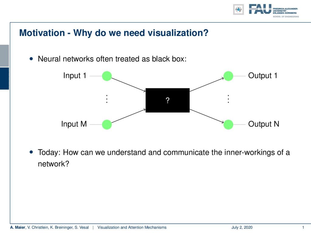
So, let’s talk a bit about motivation. Well, why do we want to visualize anything? Well of course the neural networks are often treated as black boxes. so you have some inputs, then something happens with them, and then there are some outputs. Today, we want to look into how to communicate the inner workings of a network to other people like other developers or scientists. You will see that this is an important skill that you will need for your future career.
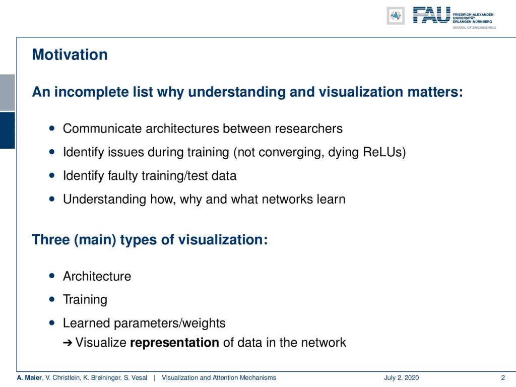
So well a couple of reasons why you want to do that. You want to communicate the architectures. You want to identify issues during the training such as if the training doesn’t converge. If you have effects like dying ReLUs, you want to identify faulty training or test data. You want to understand how why and what networks learn. So, there are three main types of visualization that we want to cover here. This is the visualization of the architecture, the visualization of the training, the learned parameters, and weights, and this is then important, of course, for visualization: The representation of the data in the network.
So, let’s start with network architecture visualization. We essentially want to communicate effectively what is important about this specific type of neural network. The priors that we actually imposed by the architecture may be crucial or even the most important factor for the good performance of a specific network. So mostly this is done graph-based structures with different degrees of granularity you will see some examples in the following. Actually, we’ve already seen this quite often if you compare to our set of lecture videos on neural network architectures. So there are essentially three categories,
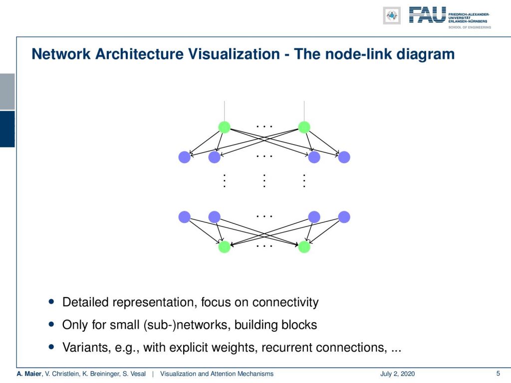
There is the node-link diagram that works essentially on neuron level. You have nodes as neurons and weighted connections as the edges. You’ve seen them especially in the early instances of this class where we really go down onto node level. There really all of the connections matter. They are, for example, useful if you want to show the difference between a convolutional layer or a fully connected layer. So, this is essentially important for small sub-networks or building blocks. There are different variants with explicit weighting recurrent connections and so on.
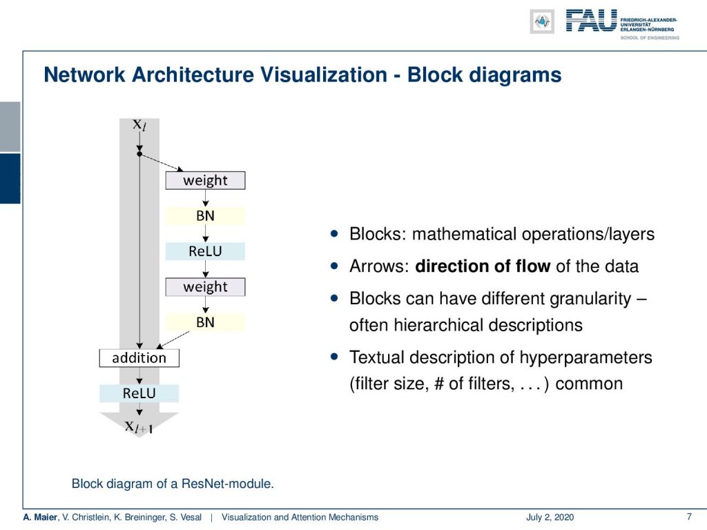
If you want to go for larger structures, then we use block diagrams. There, we have solid blocks. They often share only single connections between the layers although actually all of the neurons are connected to each other. We have seen plenty of these visualizations. Here you can see a visualization for the block diagrams. Here, the block is a mathematical operation or layer. Then, you have arrows, too. They show the flow of the data and the blocks can have different granularity. Often, they use hierarchical descriptions. You may even want to use this in combination with the previous type of diagram such that you make sure which block does what kind of operation. Of course, you need a textural description for the hyperparameters. the filter sizes. and the number of filters. This then very often is done in the caption or you add small numbers which filters are actually used or how many activations and feature maps are used.
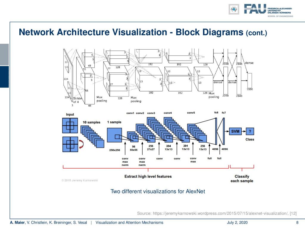
We can see there’s quite a variety of visualizations depending on what you want to show. These are two visualizations of AlexNet. The top one is actually from the original publication and it highlights that it is split into two parts because it runs on two GPUs. Then you have the interaction between the two GPUs highlighted by connections between the two branches shown on top. Now, the bottom visualization rather focuses on the convolutional neural network structure and the pooling and convolution layers. In the end, you go to fully connected layers connected to an SVM classifier. So, here more the concept of the architecture is in the focus while both of the images actually show the same architecture.
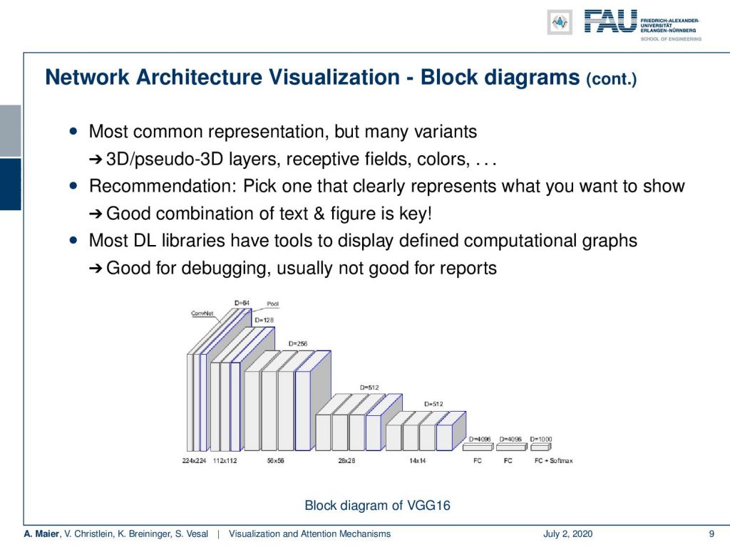
You’ve already seen that there are also block variants. So you see here the visualization of VGG where the authors wanted to show that they have this decrease in special dimensionality while an increase in the interpretation dimension. So here, only 3-D blocks or cubes are used for the visualization. Here, they convey the idea that you want to switch from the spatial dimension to the interpretation domain. There are many, many different ways of visualizing things. You should pick the one that shows the effect that is important in your opinion. Then, you add a good textural description to that one. The key is in the combination of text and figure in order for others to be able to follow your ideas. Of course, also libraries have tools that display the actually implemented graph structure. Generally, they are not so well-suited for conveying the information to others. Many details are lost or sometimes the grade of granularity is just too high in order to show the entire network. So, this is typically good for debugging, but not so good for reports or conveying the idea of your architecture.
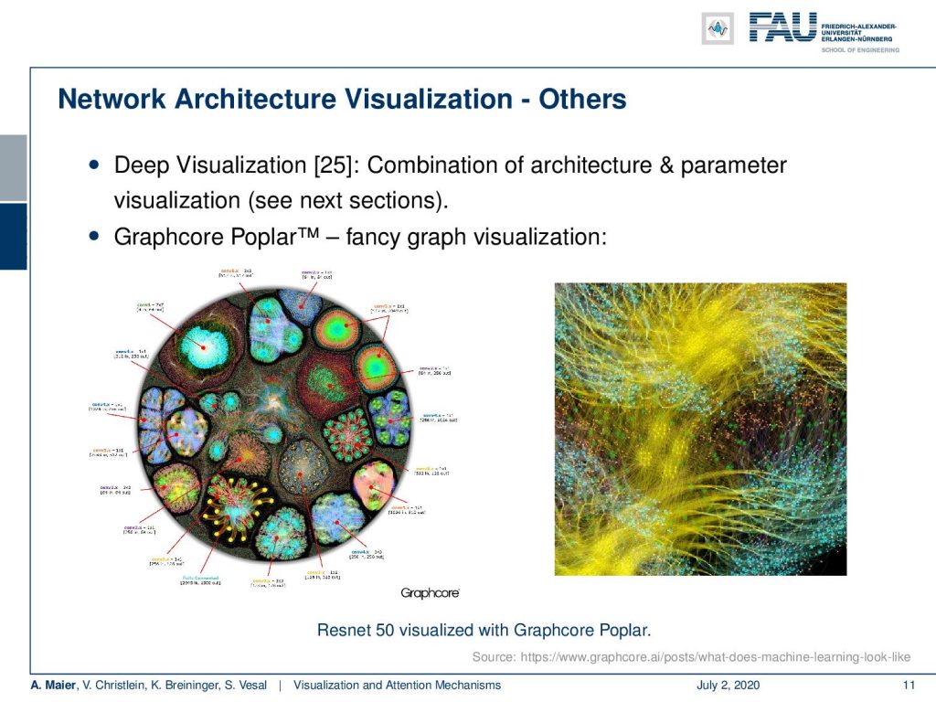
Well, there are of course also other visualization strategies. Here, we just have a short overview of what can be done. There are things like Graphcore Poplar which has this fancy graph visualization. You can see that this is a representation of the architecture but it’s not so useful if you try to implement it after this visualization, It is kind of interesting to look at it and to try to understand which part of the network is connected to which one. You can clearly see that the layers can be identified here. So, the different layers and configuration of layers form different shapes. Generally, it’s very hard to look at this image and say okay wow this is a ResNet-50. I would prefer a different visualization of ResNet-50 in order to figure out what’s going on here.
Well, let’s go ahead and talk a bit about the visualization of the training. This is also very crucial because it has lots of interesting information like the input data images, text, the parameters, the weights, the biases, the hidden layer data, or the output data.

Of course, you want to track somehow what happens during the training. So, this tracking helps in particular for debugging and improving the model design. We talked about these effects already in the lecture video series about common practices.
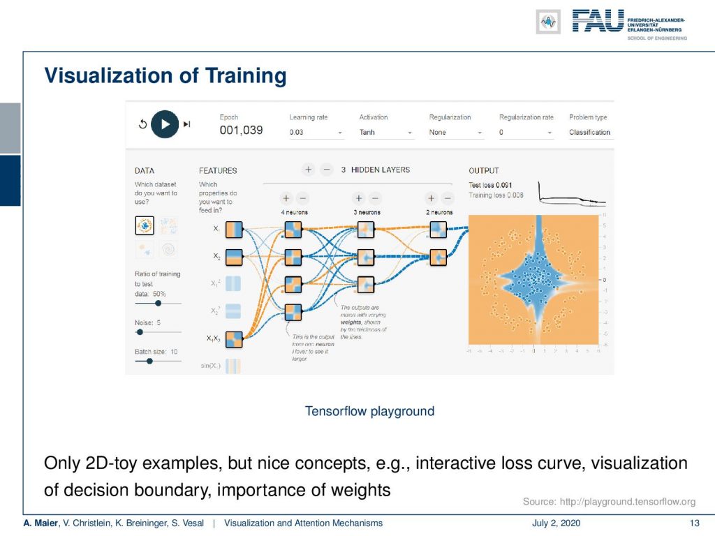
So, here is a very nice visualization of training shown in the Tensorflow playground. This is a very interesting tool because here you can not just visualize the connections, but you can also visualize the activations of a 2-D input in terms of the input space. If you go back to the very first videos you see that we actually used similar representations when we were talking for example about the tree structures. So here, you can see during the training iterations, how the representations in the different layers change. They do that by a visualization of the division that is created by the respective activation function in the input space. So, you can see the first layers using fully connected layers and sigmoid activation functions. They essentially generate binary partitions of the input space. Then, you combine the layers over the layers. You see how these different partitions of the input space can then be assembled to form a more complex shape as you can see here on the right-hand side. This is typically limited to 2-D toy examples, but it’s very nice to follow the concepts and to actually understand what’s happening during the training. You can run a couple of iterations. You can accelerate, decelerate, stop the training process, and then look at what has been happening in the different steps of the training. So, this is nice.
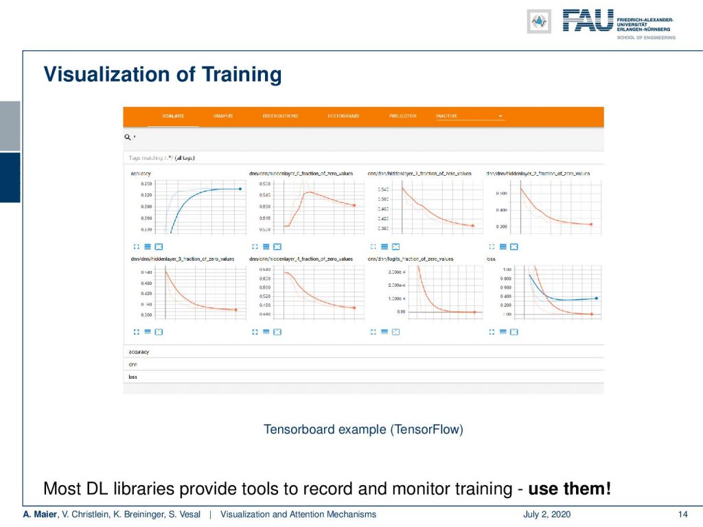
But if you want to really look into large problems, then things like Tensorboard are really useful. Here, you can monitor the actual progress during the training. This is definitely something you should use when you train large networks. Here, you can see how the loss is behaving on the training, how is the validation loss changes, and so on. You can visualize this over the entire training and you can really use that to see if there’s convergence or to detect if there’s something wrong with your training process. If you already ran like a hundred epochs and nothing happened with your loss, or if you have an exploding gradient and stuff like that, you immediately see that in visualizations of Tensorboard.
Okay. So now, we already discussed several different visualizations, in particular of the architectures and the training process. Actually, we’ve been using this all the time. Still, I think you should be aware that the way how you visualize things. This is very important if you want to convey your ideas to other people. What we’ll talk about in the next video is actually then visualizing the inner workings of the network. So, we will look into techniques on how to figure out what’s going on inside of the network. These are actually quite interesting techniques that are also very useful for debugging and trying to understand what’s happening in your network. We will start in the first video with a short motivation and some weaknesses of deep neural networks that you should be aware of. So, thank you very much for listening and see you in the next video. Bye-bye!
If you liked this post, you can find more essays here, more educational material on Machine Learning here, or have a look at our Deep LearningLecture. I would also appreciate a follow on YouTube, Twitter, Facebook, or LinkedIn in case you want to be informed about more essays, videos, and research in the future. This article is released under the Creative Commons 4.0 Attribution License and can be reprinted and modified if referenced. If you are interested in generating transcripts from video lectures try AutoBlog.
Links
Yosinski et al.: Deep Visualization Toolbox
Olah et al.: Feature Visualization
Adam Harley: MNIST Demo
References
[1] Dzmitry Bahdanau, Kyunghyun Cho, and Yoshua Bengio. “Neural Machine Translation by Jointly Learning to Align and Translate”. In: 3rd International Conference on Learning Representations, ICLR 2015, San Diego, 2015.
[2] T. B. Brown, D. Mané, A. Roy, et al. “Adversarial Patch”. In: ArXiv e-prints (Dec. 2017). arXiv: 1712.09665 [cs.CV].
[3] Jianpeng Cheng, Li Dong, and Mirella Lapata. “Long Short-Term Memory-Networks for Machine Reading”. In: CoRR abs/1601.06733 (2016). arXiv: 1601.06733.
[4] Jacob Devlin, Ming-Wei Chang, Kenton Lee, et al. “BERT: Pre-training of Deep Bidirectional Transformers for Language Understanding”. In: CoRR abs/1810.04805 (2018). arXiv: 1810.04805.
[5] Neil Frazer. Neural Network Follies. 1998. URL: https://neil.fraser.name/writing/tank/ (visited on 01/07/2018).
[6] Ross B. Girshick, Jeff Donahue, Trevor Darrell, et al. “Rich feature hierarchies for accurate object detection and semantic segmentation”. In: CoRR abs/1311.2524 (2013). arXiv: 1311.2524.
[7] Alex Graves, Greg Wayne, and Ivo Danihelka. “Neural Turing Machines”. In: CoRR abs/1410.5401 (2014). arXiv: 1410.5401.
[8] Karol Gregor, Ivo Danihelka, Alex Graves, et al. “DRAW: A Recurrent Neural Network For Image Generation”. In: Proceedings of the 32nd International Conference on Machine Learning. Vol. 37. Proceedings of Machine Learning Research. Lille, France: PMLR, July 2015, pp. 1462–1471.
[9] Nal Kalchbrenner, Lasse Espeholt, Karen Simonyan, et al. “Neural Machine Translation in Linear Time”. In: CoRR abs/1610.10099 (2016). arXiv: 1610.10099.
[10] L. N. Kanal and N. C. Randall. “Recognition System Design by Statistical Analysis”. In: Proceedings of the 1964 19th ACM National Conference. ACM ’64. New York, NY, USA: ACM, 1964, pp. 42.501–42.5020.
[11] Andrej Karpathy. t-SNE visualization of CNN codes. URL: http://cs.stanford.edu/people/karpathy/cnnembed/ (visited on 01/07/2018).
[12] Alex Krizhevsky, Ilya Sutskever, and Geoffrey E Hinton. “ImageNet Classification with Deep Convolutional Neural Networks”. In: Advances In Neural Information Processing Systems 25. Curran Associates, Inc., 2012, pp. 1097–1105. arXiv: 1102.0183.
[13] Thang Luong, Hieu Pham, and Christopher D. Manning. “Effective Approaches to Attention-based Neural Machine Translation”. In: Proceedings of the 2015 Conference on Empirical Methods in Natural Language Lisbon, Portugal: Association for Computational Linguistics, Sept. 2015, pp. 1412–1421.
[14] A. Mahendran and A. Vedaldi. “Understanding deep image representations by inverting them”. In: 2015 IEEE Conference on Computer Vision and Pattern Recognition (CVPR). June 2015, pp. 5188–5196.
[15] Andreas Maier, Stefan Wenhardt, Tino Haderlein, et al. “A Microphone-independent Visualization Technique for Speech Disorders”. In: Proceedings of the 10th Annual Conference of the International Speech Communication Brighton, England, 2009, pp. 951–954.
[16] Volodymyr Mnih, Nicolas Heess, Alex Graves, et al. “Recurrent Models of Visual Attention”. In: CoRR abs/1406.6247 (2014). arXiv: 1406.6247.
[17] Chris Olah, Alexander Mordvintsev, and Ludwig Schubert. “Feature Visualization”. In: Distill (2017). https://distill.pub/2017/feature-visualization.
[18] Prajit Ramachandran, Niki Parmar, Ashish Vaswani, et al. “Stand-Alone Self-Attention in Vision Models”. In: arXiv e-prints, arXiv:1906.05909 (June 2019), arXiv:1906.05909. arXiv: 1906.05909 [cs.CV].
[19] Mahmood Sharif, Sruti Bhagavatula, Lujo Bauer, et al. “Accessorize to a Crime: Real and Stealthy Attacks on State-of-the-Art Face Recognition”. In: Proceedings of the 2016 ACM SIGSAC Conference on Computer and Communications CCS ’16. Vienna, Austria: ACM, 2016, pp. 1528–1540. A.
[20] K. Simonyan, A. Vedaldi, and A. Zisserman. “Deep Inside Convolutional Networks: Visualising Image Classification Models and Saliency Maps”. In: International Conference on Learning Representations (ICLR) (workshop track). 2014.
[21] J.T. Springenberg, A. Dosovitskiy, T. Brox, et al. “Striving for Simplicity: The All Convolutional Net”. In: International Conference on Learning Representations (ICRL) (workshop track). 2015.
[22] Dmitry Ulyanov, Andrea Vedaldi, and Victor S. Lempitsky. “Deep Image Prior”. In: CoRR abs/1711.10925 (2017). arXiv: 1711.10925.
[23] Ashish Vaswani, Noam Shazeer, Niki Parmar, et al. “Attention Is All You Need”. In: CoRR abs/1706.03762 (2017). arXiv: 1706.03762.
[24] Kelvin Xu, Jimmy Ba, Ryan Kiros, et al. “Show, Attend and Tell: Neural Image Caption Generation with Visual Attention”. In: CoRR abs/1502.03044 (2015). arXiv: 1502.03044.
[25] Jason Yosinski, Jeff Clune, Anh Mai Nguyen, et al. “Understanding Neural Networks Through Deep Visualization”. In: CoRR abs/1506.06579 (2015). arXiv: 1506.06579.
[26] Matthew D. Zeiler and Rob Fergus. “Visualizing and Understanding Convolutional Networks”. In: Computer Vision – ECCV 2014: 13th European Conference, Zurich, Switzerland, Cham: Springer International Publishing, 2014, pp. 818–833.
[27] Han Zhang, Ian Goodfellow, Dimitris Metaxas, et al. “Self-Attention Generative Adversarial Networks”. In: Proceedings of the 36th International Conference on Machine Learning. Vol. 97. Proceedings of Machine Learning Research. Long Beach, California, USA: PMLR, Sept. 2019, pp. 7354–7363. A.