Lecture Notes in Deep Learning: Recurrent Neural Networks – Part 5

Sequence Generation

These are the lecture notes for FAU’s YouTube Lecture “Deep Learning“. This is a full transcript of the lecture video & matching slides. We hope, you enjoy this as much as the videos. Of course, this transcript was created with deep learning techniques largely automatically and only minor manual modifications were performed. Try it yourself! If you spot mistakes, please let us know!

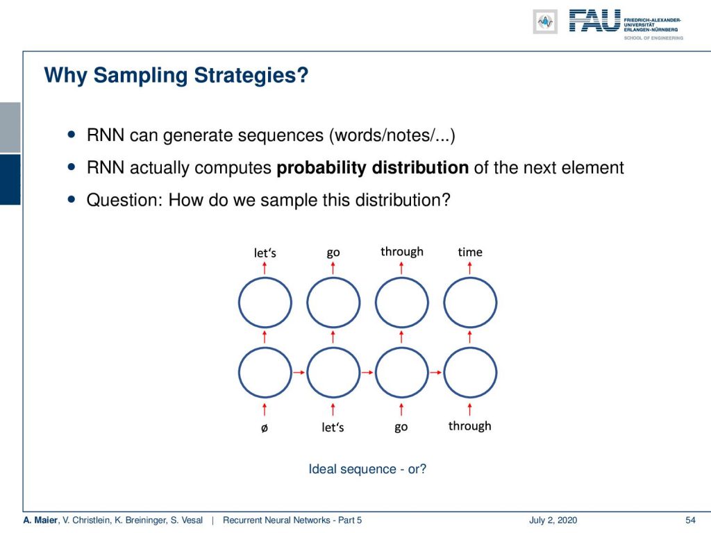
Welcome back to the final part of our video series on recurrent neural networks! Today, we want to talk a bit about the sampling of recurrent neural networks. When I mean sampling, I mean that we want to use recurrent neural networks to actually generate sequences of symbols. So, how can we actually do that?

Well, if you train your neural networks in the right way. You can actually create them in a way that they predict the probability distribution of the next element. So, if I train them to predict the next symbol in the sequence, you can also use them actually for generating sequences. The idea here is that you start with the empty symbol and then you use the RNN to generate some output. Then, you take this output and put it into the next state’s input. If you go ahead and do so, then you can see that you can actually generate whole sequences from your trained recurrent neural network.

So, the simple strategy is to perform a greedy search. So here we start with the empty symbol. Then, we just pick the most likely element as the input to the RNN in the next state and generate the next one and the next one and the next one and this generates exactly one sample sequence per experiment. So, this would be a greedy search and you can see that we exactly get one sentence that is constructed here. The sentence that we are constructing here is “let’s go through time”. Well, the drawback is, of course, there is no look-ahead possible. So, let’s say the most likely word after “let’s go” is “let’s”. So you could be generating loops like “let’s go let’s go” and so on. So, you’re not able to detect that “let’s go through time” has a higher total probability. So, it tends to repeat sequences of frequent words “and”, “the”, “some” and so on in speech.

Now, we are interested in alleviating this problem. This can be done with a beam search. Now, the beam search concept is to select the k most likely elements. k is essentially the beam width or size. So, here you then roll out k possible sequences. You have the one with these k elements as prefix and take the k most probable ones. So, in the example that we show here on the right-hand side, we start with the empty word. Then, we take the two most likely ones which would be “let’s” and “through”. Next, we generate “let’s” as output if we take “through”. If we take “let’s”, we generate “go” and we can continue this process and with our beam of the size of two. We can keep the two most likely sequences in the beam search. So now, we generate two sequences at a time. One is “let’s go through time” and the other one is “through let’s go time”. So, you see that we can use this beam idea to generate multiple sequences. In the end, we can determine which one we like best or which one generated the most total probability. So, we can generate multiple sequences in one go which typically then also contains better sequences than in the greedy search. I would say this is one of the most common techniques actually to sample from an RNN.

Of course, there are also other things like random sampling. Here, the idea is that you select the next one according to the output probability distribution. You remember, we encoded our word as one-hot-encoded vectors. Then, we can essentially interpret the output of the RNN as a probability distribution and sample from it. This then allows us to generate many different sequences. So let’s say if “let’s” has an output probability of 0.8, it is sampled 8 out of 10 times as the next word. This creates very diverse results and it may look too random. So, you see here we get quite diverse results and the sequences that we are generating here. There’s quite some randomness that you can also observe in the generated sequences. To reduce the randomness, you can increase the probability or decrease the probability of probable or less probable words. This can be done for example by temperature sampling. Here you see that we introduced this temperature 𝜏 that we then use in order to steer the probability sampling. This is a common technique that you have already seen in various instances in this class.

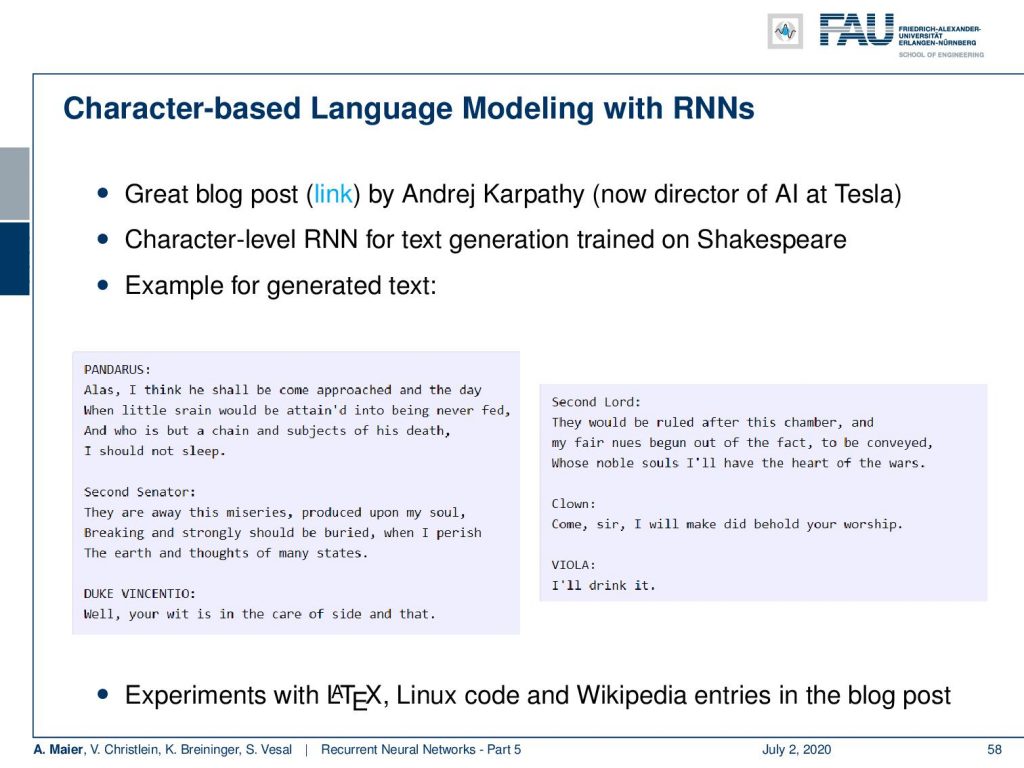
So let’s look into some examples and one thing that I found very interesting is character-based language modeling with RNNs. There’s a great blog post by Andrew Kaparthy which we have here. I also put it as a link to the description below. There he essentially trained an RNN for text generation based on Shakespeare. It’s trained on the character level. So, you only have one character as input and then you generate the sequence. It generates very interesting sequences. So here, you can see typical examples that have been generated. Let me read this to you:

“Pandarus
Alas I think he shall be come approached and the day
When little srain would be attain’d into being never fed,
And who is but a chain and subjects of his death,
I should not sleep.”

Except from Karparthy’s blog

and so on. So, you can see that this is very interesting that the type of language that is generated this very close to Shakespeare but if you read through these examples, you can see that they’re essentially complete nonsense. Still, it’s interesting that the tone of the language that is generated is still present and is very typical for Shakespeare. So, that’s really interesting.

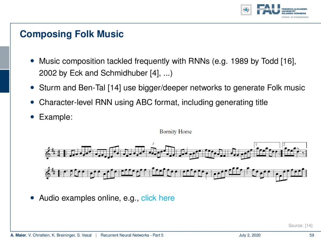
Of course, you can generate many, many other things. One of a very nice example that I want to show to you today is composing folk music. So, music composition is typically tackled with RNNS and you can find different examples in literature, also by Jürgen Schmidhuber. The idea here is to use bigger deeper networks to generate folk music. So, what they employ is a character level RNN using ABC format including generating the title. So one example that I have here is this small piece of music. Yeah, as you can hear, it is really folk music. So, this is completely automatically generated. Interesting isn’t it? If you listen very closely, then you can also hear that folk music may be particularly suited for this because you could argue it’s kind a bit of repetitive. Still, it’s pretty awesome that the entire song is completely automatically generated. There are actually people meeting playing computer-generated songs like these folks on real instruments. Very interesting observation. So, I also put the link here for your reference if you’re interested in this. You can listen to many more examples on this website.

So there are also RNNs for non-sequential tasks. RNNs can also be used for stationary inputs like image generation. Then, the idea is to model the process from rough sketch to final image. You can see one example here where we start essentially by drawing numbers from blurry to sharp. In this example, they use an additional attention mechanism telling the network where to look. This then generates something similar to brushstrokes. It actually uses a variational autoencoder which we will talk about when we talk on the topic of unsupervised deep learning.

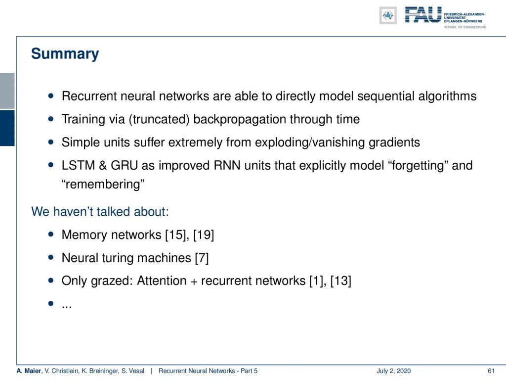
So let’s summarize this a little bit. You’ve seen recurrent neural networks are able to directly model sequential algorithms. You train via truncated backpropagation through time. The simple units suffer extremely from the exploding and vanishing gradients. We have seen that the LSTMs and GRUs are improved RNNs that explicitly model this forgetting and remembering operation. What we haven’t talked about is that there are many, many more developments that we can’t cover in this short lecture. So, it would be interesting also to talk about memory networks, neural Turing machines, and what we only touched at the moment is attention and recurrent neural networks. We’ll talk a bit more about attention in one of the next videos as well.

So, next time in deep learning, we want to talk about visualization. In particular, we want to talk about visualizing architectures the training process, and of course also the inner workings of the network. We want to figure out what is actually happening inside the network and there are quite a few techniques – and to be honest – we’ve already seen some of them earlier in this class. In this lecture, we will really want to look into those methods and understand how they actually work in order to figure out what’s happening inside of deep neural networks. One interesting observation is that this is also related to neural network art. Another thing that deserves some little more thought is attention mechanisms and this will also be covered in one of the videos very soon to follow.

So, I have some comprehensive questions: “What’s the strength of RNNs compared to feed-forward networks?” Then, of course: “How do you train an RNN?”, “What are the challenges?”, “What’s the main idea behind LSTMs?” So you should be able to describe the unrolling of RNNs during the training. You should be able to describe the Elman cell, the LSTM, and the GRU. So, these are really crucial things that you should know if you have to take some tests in the very close future. So, better be prepared for questions like this one. Ok, we have some further reading below. There’s this very nice blog post by Andrew Kaparthy. There is a very cool blog post about CNN’s for a machine translation that I really recommend reading and a cool blog post for music generation which you can also find below. Of course, we also have plenty of scientific references. So, I hope you enjoyed this video and see you in the next one. Bye-bye!

If you liked this post, you can find more essays here, more educational material on Machine Learning here, or have a look at our Deep LearningLecture. I would also appreciate a follow on YouTube, Twitter, Facebook, or LinkedIn in case you want to be informed about more essays, videos, and research in the future. This article is released under the Creative Commons 4.0 Attribution License and can be reprinted and modified if referenced. If you are interested in generating transcripts from video lectures try AutoBlog.

RNN Folk Music

FolkRNN.org
MachineFolkSession.com
The Glass Herry Comment 14128

Links

Character RNNs
CNNs for Machine Translation
Composing Music with RNNs

References

[1] Dzmitry Bahdanau, Kyunghyun Cho, and Yoshua Bengio. “Neural Machine Translation by Jointly Learning to Align and Translate”. In: CoRR abs/1409.0473 (2014). arXiv: 1409.0473.
[2] Yoshua Bengio, Patrice Simard, and Paolo Frasconi. “Learning long-term dependencies with gradient descent is difficult”. In: IEEE transactions on neural networks 5.2 (1994), pp. 157–166.
[3] Junyoung Chung, Caglar Gulcehre, KyungHyun Cho, et al. “Empirical evaluation of gated recurrent neural networks on sequence modeling”. In: arXiv preprint arXiv:1412.3555 (2014).
[4] Douglas Eck and Jürgen Schmidhuber. “Learning the Long-Term Structure of the Blues”. In: Artificial Neural Networks — ICANN 2002. Berlin, Heidelberg: Springer Berlin Heidelberg, 2002, pp. 284–289.
[5] Jeffrey L Elman. “Finding structure in time”. In: Cognitive science 14.2 (1990), pp. 179–211.
[6] Jonas Gehring, Michael Auli, David Grangier, et al. “Convolutional Sequence to Sequence Learning”. In: CoRR abs/1705.03122 (2017). arXiv: 1705.03122.
[7] Alex Graves, Greg Wayne, and Ivo Danihelka. “Neural Turing Machines”. In: CoRR abs/1410.5401 (2014). arXiv: 1410.5401.
[8] Karol Gregor, Ivo Danihelka, Alex Graves, et al. “DRAW: A Recurrent Neural Network For Image Generation”. In: Proceedings of the 32nd International Conference on Machine Learning. Vol. 37. Proceedings of Machine Learning Research. Lille, France: PMLR, July 2015, pp. 1462–1471.
[9] Kyunghyun Cho, Bart Van Merriënboer, Caglar Gulcehre, et al. “Learning phrase representations using RNN encoder-decoder for statistical machine translation”. In: arXiv preprint arXiv:1406.1078 (2014).
[10] J J Hopfield. “Neural networks and physical systems with emergent collective computational abilities”. In: Proceedings of the National Academy of Sciences 79.8 (1982), pp. 2554–2558. eprint: http://www.pnas.org/content/79/8/2554.full.pdf.
[11] W.A. Little. “The existence of persistent states in the brain”. In: Mathematical Biosciences 19.1 (1974), pp. 101–120.
[12] Sepp Hochreiter and Jürgen Schmidhuber. “Long short-term memory”. In: Neural computation 9.8 (1997), pp. 1735–1780.
[13] Volodymyr Mnih, Nicolas Heess, Alex Graves, et al. “Recurrent Models of Visual Attention”. In: CoRR abs/1406.6247 (2014). arXiv: 1406.6247.
[14] Bob Sturm, João Felipe Santos, and Iryna Korshunova. “Folk music style modelling by recurrent neural networks with long short term memory units”. eng. In: 16th International Society for Music Information Retrieval Conference, late-breaking Malaga, Spain, 2015, p. 2.
[15] Sainbayar Sukhbaatar, Arthur Szlam, Jason Weston, et al. “End-to-End Memory Networks”. In: CoRR abs/1503.08895 (2015). arXiv: 1503.08895.
[16] Peter M. Todd. “A Connectionist Approach to Algorithmic Composition”. In: 13 (Dec. 1989).
[17] Ilya Sutskever. “Training recurrent neural networks”. In: University of Toronto, Toronto, Ont., Canada (2013).
[18] Andrej Karpathy. “The unreasonable effectiveness of recurrent neural networks”. In: Andrej Karpathy blog (2015).
[19] Jason Weston, Sumit Chopra, and Antoine Bordes. “Memory Networks”. In: CoRR abs/1410.3916 (2014). arXiv: 1410.3916.

Category: Lecture Notes in Deep Learning