
Policy Iteration
These are the lecture notes for FAU’s YouTube Lecture “Deep Learning“. This is a full transcript of the lecture video & matching slides. We hope, you enjoy this as much as the videos. Of course, this transcript was created with deep learning techniques largely automatically and only minor manual modifications were performed. Try it yourself! If you spot mistakes, please let us know!

Welcome back to deep learning! So today, we want to go deeper into reinforcement learning. The concept that we want to explain today is going to be policy iteration. It tells us how to make better policies towards designing strategies for winning games.
So, let’s have a look at the slides that I have here for you. So it’s the third part of our lecture and we want to talk about policy iteration. Now, before we had this action-value function that somehow could assess the value of an action. Of course, this now has also to depend on the state t. This is essentially our – you could say Oracle – that tries to predict the future reward g subscript t. It depends on following a certain policy that describes how to select the action and the resulting state. Now, we can also find an alternative formulation here. We introduce the state-value function. So, previously we had the action-value function that told us how valuable a certain action is. Now, we want to introduce the state-value function that tells us how valuable a certain state is. Here, you can see that it is formalized in a very similar way. Again, we have some expected value over our future reward. This is now, of course, dependent on the state. So, we kind of leave away the dependency on the action and we only focus on the state. You can now see that this is the expected value of the future reward with respect to the state. So, we want to marginalize the actions. We don’t care about what the influence of the action is. We just want to figure out what the value of a certain state is.
We can actually compute this. So, we can also do this for our grid example. If you recall this one, you remember that we had the simple game where you had A and B that were essentially the locations on the grid that would then teleport you to A’ and B’. Once, you arrive at A’ and B’, you get a reward. For A’ its +10 and for B’ it’s +5. Whenever you try to leave the board, you get a negative reward. Now, we can play this game and compute the state-value function. Of course, we can do this under the uniform random policy because we don’t have to know anything about the game. If we play the random uniform policy, we can simply choose actions, play this game for a certain time, and then we are able to compute these state values according to the previous definition. You can see that the edge tiles, in particular, in the bottom, they even have a negative value. Of course, they can have negative values because if you are in the edge tiles, we find -1.9 and -2.0 and the bottom. At the corner tiles, there is a 50% likelihood that you will try to leave the grid. In these two directions, you will, of course, generate a negative reward. So, you can see that we have states that are much more valuable. You can see if you look at the positions where A and B are located, they have a very high value. So A has an expected future reward of 8.8 and the tile with B has an expected future reward of 5.3. So, these are really good states. So, you could say with this state value, we have somehow learned something about our game. So, you could say “Okay, maybe we can use this.” We can now use the greedy action selection on this state value. So let’s define a policy and this policy is now selecting always the action that leads into a state of a higher value. If you do so, you have a new policy. If you play with this new policy you see you have a better policy.
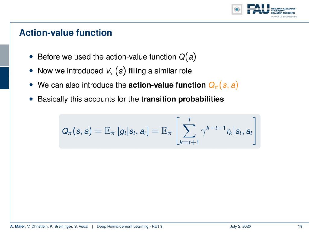
So, we can now relate this to the action-value function that we used before. We somehow introduced the state-value function in a similar role. So, we can now see that we can introduce an action-value function that is Q subscript policy of s and a, i.e., of the state and the action. This then basically accounts for the transition probabilities. So, you can now compute your Q policy of state and action as the expected value of the future rewards given the state and the action. You can compute this in a similar way. Now, you get an expected future reward for every state and for every action.
Are all of these value functions created equal? No. There can only be one optimal state value function. We can show its existence without referring to a specific policy. So, the optimal state-value function is simply the maximum of all state-value functions with the best policy. So, the best policy will always produce the optimal state-value function. Now, we can also define the optimal action-value function. This can now be related to our optimal state-value function. We can see that the optimal action-value function is given as the expected reward in the next step plus our discount factor times the optimal state-value function. So, if we know the optimal state-value function, then we can also derive the optimal action-value function. So, they are related to each other.
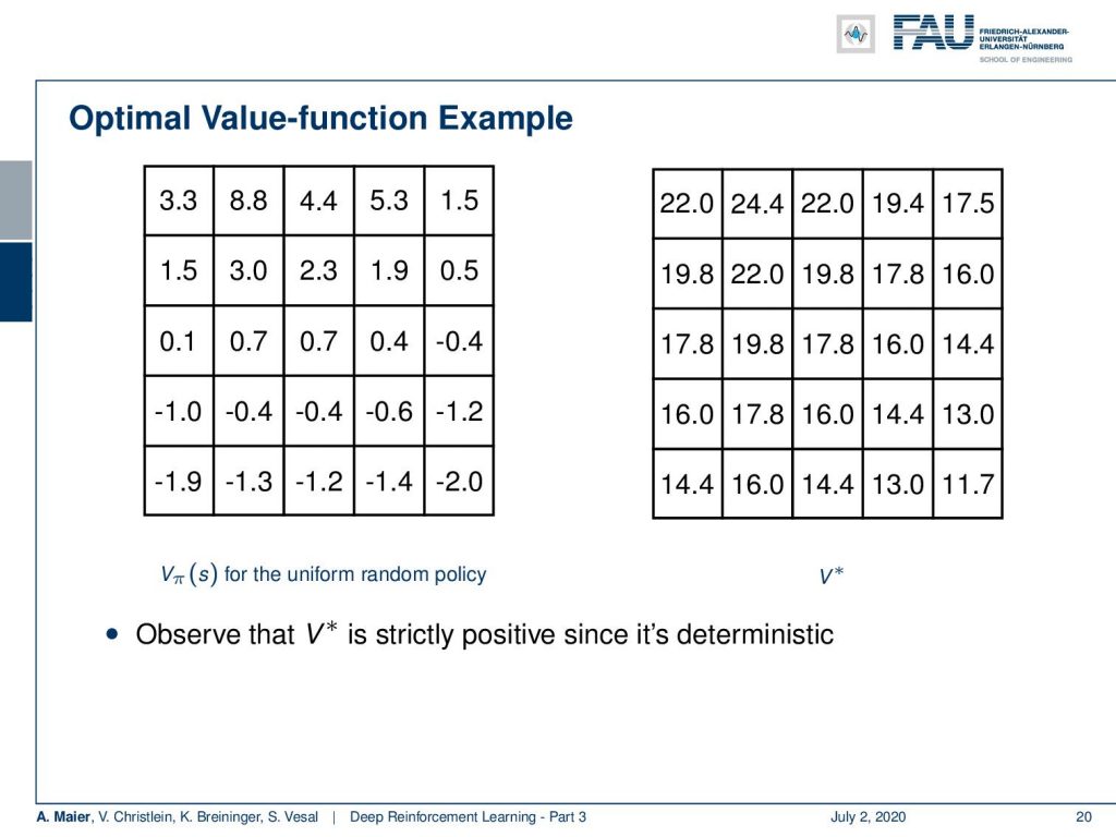
So, this was the state-value function for the uniform random policy. I can show you the optimal V*, i.e., the optimal state-value function. You see that this has much higher values, of course, because we have been optimizing for this. You also observe that the optimal state-value function is strictly positive because we are in a deterministic setting here. So, very important observation: In a deterministic setting, the optimal state-value function will be strictly positive.
Now, we can also order policies. We have to determine what is a better policy. We can order them with the following concept: A better policy π is better than a policy π’ if and only if the state values of π are all higher than the state values that you obtain with π’ for all states in the set of states. If you do this, then any policy that returns the optimal state-value function is an optimal policy. So, you see that it’s only one optimal state-value function, but there might be more than one optimal policy. So, there could be two or three different policies that result in the same optimal state-value function. So, if you know either the optimal state-value or the optimal action-value function, then you can directly obtain an optimal policy by greedy action selection. So, if you know the optimal state values and if you have complete knowledge about all the actions and so on, then you can always get the optimal policy by a greedy action selection.
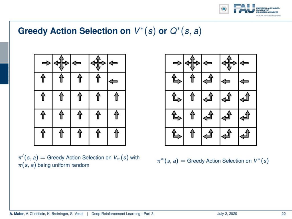
So, let’s have a look at how this would then actually result in terms of policies. Now, greedy action selection on the optimum state-value function or the optimal action-value function would lead to the optimal policy. Well, you see here on the left inside is greedy action selection on the uniform random state-value function. So, what we’ve computed earlier in this video. You can, of course, choose your action in a way that you have the next state being a state of higher value and you end up with this kind of policy. Now, if you do the same thing on the optimal state value function, you can see that we essentially emerge with a very similar policy. You see a couple of differences. In fact, you don’t always have to move up like shown on the left-hand side. So, you can also move left or up on several occasions. You can actually choose the action at each of these squares that are indicated with multiple arrows with equal probability. So, if there’s an up and left arrow, you can choose either action and you would still have an optimal policy. So, this would be the optimal policy that is created by a greedy action selection on the optimal state value function.
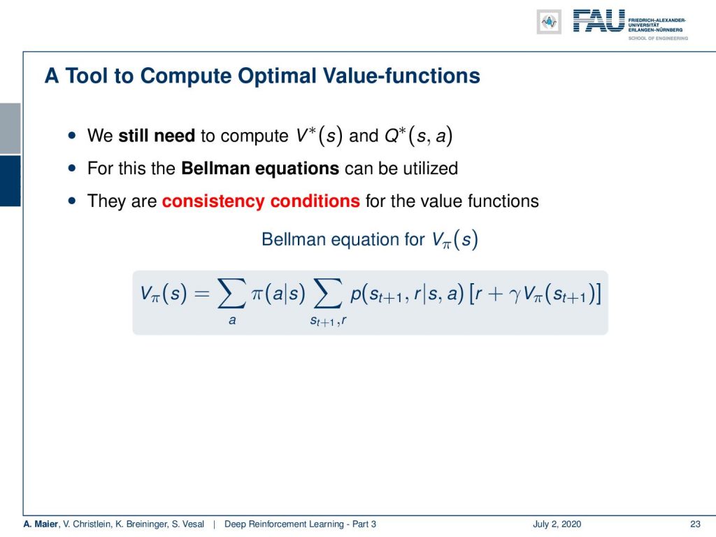
Now, the big question is: “How can we compute optimal value functions?” We still have to determine this optimal state-value function and the optimal action-value function. In order to do this, there are the Bellman equations. They are essentially consistency conditions for value functions. So, this is the example of the state-value function. You can see that you have to sum over all the different actions that are determined by your policy. So, we want to marginalize out the influence of the actual action. Of course, depending on what action you would choose, you would generate different states and different rewards. So, you also sum over the different states and the respective rewards here and multiply the probability of the states with the actual reward plus the discounted state-value function of the next state. So in this way, you can determine the state-value function. You see that there is this dependency between the current state and the next state in this computation.
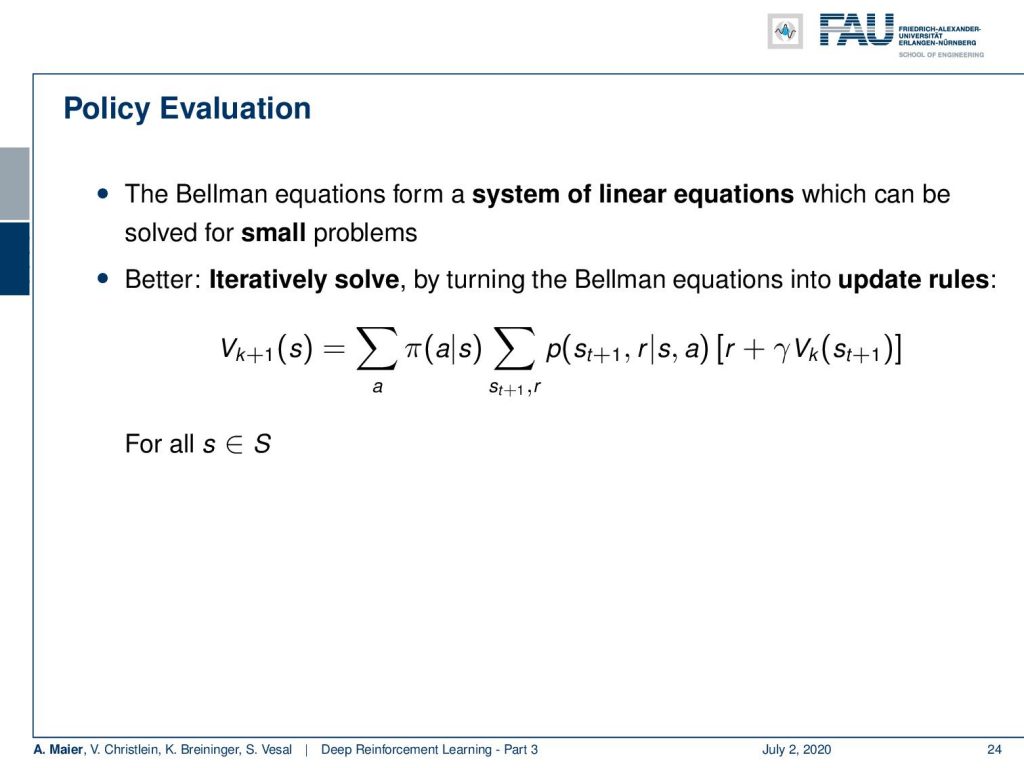
This means you can either write this up as a system of linear equations and actually solve this for small problems. But what is even better is that you iteratively solve this by turning the Bellman equations into update rules. So, you see now that we can generate a new value function k+1 for the current state if we simply apply the Bellman equation. So, we have to compute all of the different actions. We have to evaluate actually all of the different actions given the state. Then, we determine all the next future states and the next future rewards and update this according to our previous state-value function. Of course, we do this for all the states s. Then, we have an updated state-value function. Okay. So, this is an interesting observation. If we have some policy, we can actually run those updates.
This leads us then to the concept of policy improvement. This policy iteration is what we actually want to talk about in this video. So, we can use now our state-value function to guide our search for good policies. Then, we update the policy. So, if we use the greedy action selection for an update of the state-value function, then this also means that we simultaneously update our policy because the greedy action selection on our state value will always result in different actions if we change the state values. So, any change or update in the state values will also imply an updated policy in case of greedy action selection because we directly linked them together. So this then means that we can iterate the evaluation of a greedy policy on our state-value function. We stop iterating if our policy stops changing. So, this way we can update the state values and with the update of the state values, we immediately also update our policy. Is this actually guaranteed to work?
Well, there’s the policy improvement theorem. If we consider changing a single action a subscript t and state s subscript t, following a policy. Then, in general, if we have a higher action-value function, the state value for all states s increases. This means that we have a better policy. So, the new policy is then a better policy. This would then also imply that we also get a better state value because we generate a higher future reward in all of the states. This means that also the state-value function must have been increased. If we only greedy select, then we will always produce a higher action value than the state value before the convergence. So, we iteratively updating the state value using greedy action selection is really a guaranteed concept here in order to improve our state values. We terminate if the policy no longer changes. One last remark: if we don’t loop over all the states in our state space for the policy evaluation but update the policy directly, this is then called value iteration. Okay. So, you have seen now in this video how we can use the state value function in order to describe the expected future reward of a specific state. We have seen that if we do greedy action selection on the state-value function, we can use this to generate better policies. If we follow a better policy, then also our state-value function will increase. So if we follow this concept, we end up in the concept of policy iteration. So with every update of the state value function where you find higher state values, you also find a better policy. This means that we can improve our policy step-by-step by the concept of policy iteration. Okay. So, this was a very first learning algorithm in the concept of reinforcement learning.
But of course, this is not everything. There are a couple of drawbacks and we’ll talk about more concepts on how to improve actually our policies in the next video. There are a couple more. So, we will present them and also talk a bit about the drawbacks of the different versions. So, I hope you liked this video and we will talk a bit more in the next couple of videos about reinforcement learning. So, stay tuned and hope to see you in the next video. Bye-bye!

If you liked this post, you can find more essays here, more educational material on Machine Learning here, or have a look at our Deep LearningLecture. I would also appreciate a follow on YouTube, Twitter, Facebook, or LinkedIn in case you want to be informed about more essays, videos, and research in the future. This article is released under the Creative Commons 4.0 Attribution License and can be reprinted and modified if referenced. If you are interested in generating transcripts from video lectures try AutoBlog.
Links
Link to Sutton’s Reinforcement Learning in its 2018 draft, including Deep Q learning and Alpha Go details
References
[1] David Silver, Aja Huang, Chris J Maddison, et al. “Mastering the game of Go with deep neural networks and tree search”. In: Nature 529.7587 (2016), pp. 484–489.
[2] David Silver, Julian Schrittwieser, Karen Simonyan, et al. “Mastering the game of go without human knowledge”. In: Nature 550.7676 (2017), p. 354.
[3] David Silver, Thomas Hubert, Julian Schrittwieser, et al. “Mastering Chess and Shogi by Self-Play with a General Reinforcement Learning Algorithm”. In: arXiv preprint arXiv:1712.01815 (2017).
[4] Volodymyr Mnih, Koray Kavukcuoglu, David Silver, et al. “Human-level control through deep reinforcement learning”. In: Nature 518.7540 (2015), pp. 529–533.
[5] Martin Müller. “Computer Go”. In: Artificial Intelligence 134.1 (2002), pp. 145–179.
[6] Richard S. Sutton and Andrew G. Barto. Introduction to Reinforcement Learning. 1st. Cambridge, MA, USA: MIT Press, 1998.