Alternative Approaches
These are the lecture notes for FAU’s YouTube Lecture “Deep Learning“. This is a full transcript of the lecture video & matching slides. We hope, you enjoy this as much as the videos. Of course, this transcript was created with deep learning techniques largely automatically and only minor manual modifications were performed. Try it yourself! If you spot mistakes, please let us know!
Welcome back to deep learning! Today we want to discuss a couple of other reinforcement learning approaches than the policy iteration concept that you’ve seen in the previous video. So let’s have a look at what I’ve got for you today. We will look at other solution methods.
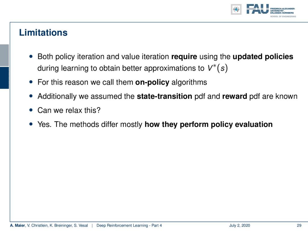
You see that in the policy and value iteration that we discussed earlier, they require updated policies during the learning to obtain better approximations of our optimal state-value function. So, these are called on policy algorithms because you need n policy. This policy is being updated. Additionally, we assumed that the state transition and the reward are known. So, the probability density functions that produce the new states and the new reward are known. If they are not then you can’t apply the previous concept. So, this very important and of course there are methods where you can then relax this. So, these methods mostly differ in how they perform the policy evaluation. So, let’s look at a couple of those alternatives.
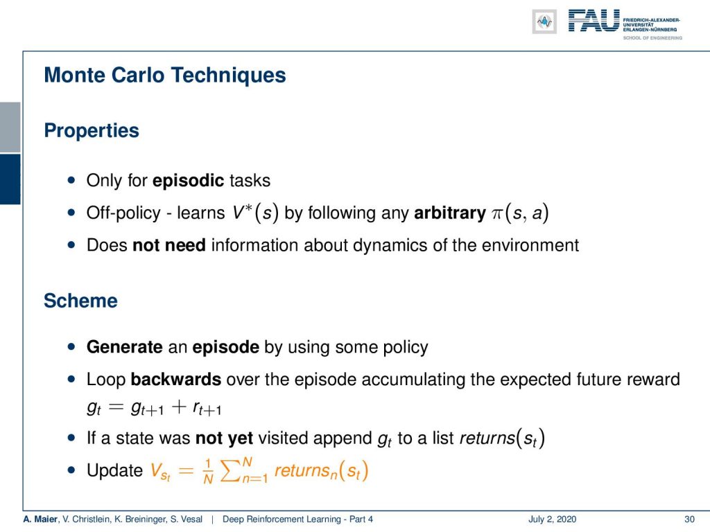
The first one that I want to show you is based on Monte Carlo techniques. This applies only to episodic tasks. Here, the idea is off-policy. So, you learn the optimal state value by following an arbitrary policy. It doesn’t matter what policy you’re using. So it’s an arbitrary policy. It could be multiple policies. Of course, you still have the exploration/exploitation dilemma. So you want to choose policies that really visit all of the states. You don’t need information about the dynamics of the environment because you can simply run many of the episodic tasks. You try to reach all of the possible states. If you do so, then you can generate those episodes using some policy. Then, you loop in backward direction over one episode and you accumulate the expected future reward. Because you have played the game until the end, you can go backward in time over this episode and accumulate the different rewards that have been obtained. If a state was not yet visited, you append it to a list and essentially you use this list then to compute the update for the state value function. So, you see this is simply the sum over these lists for that specific state. This will allow you to update your state value and this way you can then iterate in order to achieve the optimal state value function.
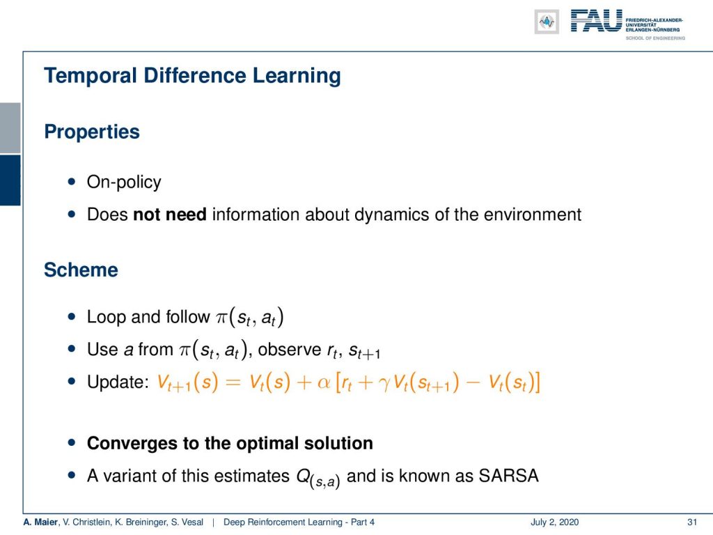
Now, another concept is temporal difference learning. This is an on-policy method. Again, it does not need information about the dynamics of the environment. So here, the scheme is that you loop and follow a certain policy. Then you use an action from the policy to observe the rewards and the new states. You update your state-value function using the previous state-value function plus α that is used to weight the influence of the new observations times the new reward plus the discounted version of the old state value function of the new state and you subtract the value of the old state. So this way, you can generate updates and this actually converges to the optimal solution. A variant of this estimates actually the action-value function and is then known as SARSA.
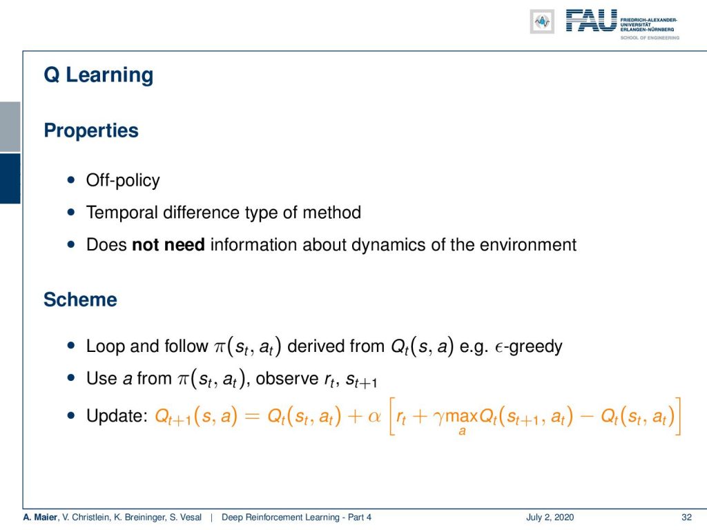
Q learning is an off-policy method. It’s a temporal difference type of method but it does not require information about the dynamics of the environment. Here, the idea is that you loop and follow a policy derived from your action-value function. For example, you could use an ε-greedy type of approach. Then, you use the action from the policy to observe your reward and your new state. Next, you update your action-value function using the previous action-value plus some weighting factor times the observed reward again the discounted action that would have derived the maximum action value over what you have already known from the state that is generated minus the action-value function of the previous state. So it’s again a kind of temporal difference that you are using here in order to update your action-value function.
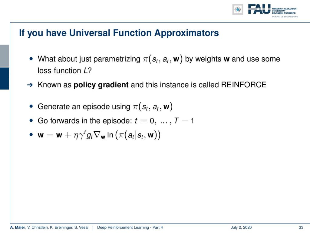
Well, if you have Universal function approximators, what about just parameterizing your policy with weights w and some loss function? This is known as the policy gradient. This instance is called REINFORCE. So, you generate an episode using your policy and your weights. Then, you go forward in your episode from time 0 to time t – 1. If you do so, you can actually compute the gradient with respect to the weights. You use this gradient in order to update your weights. Very similar way as we have previously seen in our learning approaches. You can see that this idea using the gradient over the policy then gives you an idea of how you can update the weights, again with a learning rate. We are really close to our machine learning ideas from earlier now.
This is why we talk in the next video about deep Q learning which is the kind of deep learning version of reinforcement learning. So, I hope you like this video. You’ve now seen other options on how you can actually determine the optimal state-value and action-value function. This way, we have seen that there are many different ideas that do no longer require exact knowledge on how to generate future states and on how to generate future rewards. So with these ideas, you can also do reinforcement learning and in particular the idea of the policy gradient. We’ve seen that this is very much compatible with what we’ve seen earlier in this class regarding our machine learning and deep learning methods. We will talk about exactly this idea in the next video. So thank you very much for listening and see you in the next video. Bye-bye!
If you liked this post, you can find more essays here, more educational material on Machine Learning here, or have a look at our Deep LearningLecture. I would also appreciate a follow on YouTube, Twitter, Facebook, or LinkedIn in case you want to be informed about more essays, videos, and research in the future. This article is released under the Creative Commons 4.0 Attribution License and can be reprinted and modified if referenced. If you are interested in generating transcripts from video lectures try AutoBlog.
Links
Link to Sutton’s Reinforcement Learning in its 2018 draft, including Deep Q learning and Alpha Go details
References
[1] David Silver, Aja Huang, Chris J Maddison, et al. “Mastering the game of Go with deep neural networks and tree search”. In: Nature 529.7587 (2016), pp. 484–489.
[2] David Silver, Julian Schrittwieser, Karen Simonyan, et al. “Mastering the game of go without human knowledge”. In: Nature 550.7676 (2017), p. 354.
[3] David Silver, Thomas Hubert, Julian Schrittwieser, et al. “Mastering Chess and Shogi by Self-Play with a General Reinforcement Learning Algorithm”. In: arXiv preprint arXiv:1712.01815 (2017).
[4] Volodymyr Mnih, Koray Kavukcuoglu, David Silver, et al. “Human-level control through deep reinforcement learning”. In: Nature 518.7540 (2015), pp. 529–533.
[5] Martin Müller. “Computer Go”. In: Artificial Intelligence 134.1 (2002), pp. 145–179.
[6] Richard S. Sutton and Andrew G. Barto. Introduction to Reinforcement Learning. 1st. Cambridge, MA, USA: MIT Press, 1998.