
Markov Decision Processes
These are the lecture notes for FAU’s YouTube Lecture “Deep Learning“. This is a full transcript of the lecture video & matching slides. We hope, you enjoy this as much as the videos. Of course, this transcript was created with deep learning techniques largely automatically and only minor manual modifications were performed. Try it yourself! If you spot mistakes, please let us know!
Welcome back to deep learning! So, today we want to discuss a little bit about this so-called Markov decision process which is the fundament of reinforcement learning.
I brought a couple of slides for you. We can see here what we are actually talking about. The topic is now reinforcement learning. Really, we want to learn how to play games. The key element will be the Markov decision process. So, we have to extend the multi-armed bandit problem that we talked about in the previous video. We have to introduce a state s subscript t of the world. So, the world now has a state. The rewards also depend on the action and the state of the word. So, depending on the state of the world, actions may produce a very different reward. We can encode this again in a probability density function as you can see here on the slide. What else? Well, this setting now is known as the contextual bandit. In the full reinforcement learning problem also the actions influence the state. So, we will see whatever action I take, it will also have an effect on the state and this may also be probabilistic.
So, we can describe it in another probability density function. This then leads us to the so-called Markov decision process. Markov decision processes, they take the following form: You have an agent, and the agent here on top is doing actions a subscript t. These actions have an influence on the environment which then generates rewards as in the multi-armed bandit problem. It also changes the state. So now, our actions and the state are in relation to each other and they are of course dependent. Thus, we have a state transition probability density function that will cause the state to be altered depending on the previous state and the action that was taken. This transition also produces a reward and this reward is now dependent on the state and the action. Otherwise, it’s very similar to what we’ve already seen in the multi-armed bandit problem. Of course, we need policies, and the policies now also get the dependency on the state because you want to look into the state in order to pick your action and not just rely on the prior knowledge to choose the actions independent of the state. So, all of them are expanded accordingly. Now, if all of these sets are finite this is a finite Markov decision process. If you look at this figure, you can see this is a very abstract way of describing the entire situation. The agent is essentially the system that chooses the actions and designs the actions. The environment is everything else. So, for example, if you were to control a robot, the robot itself would probably be part of the environment as the location of the robot is also encoded in the state. Everything that can be done by the agent is merely designing actions. The knowledge about the current situation is encoded in the state.
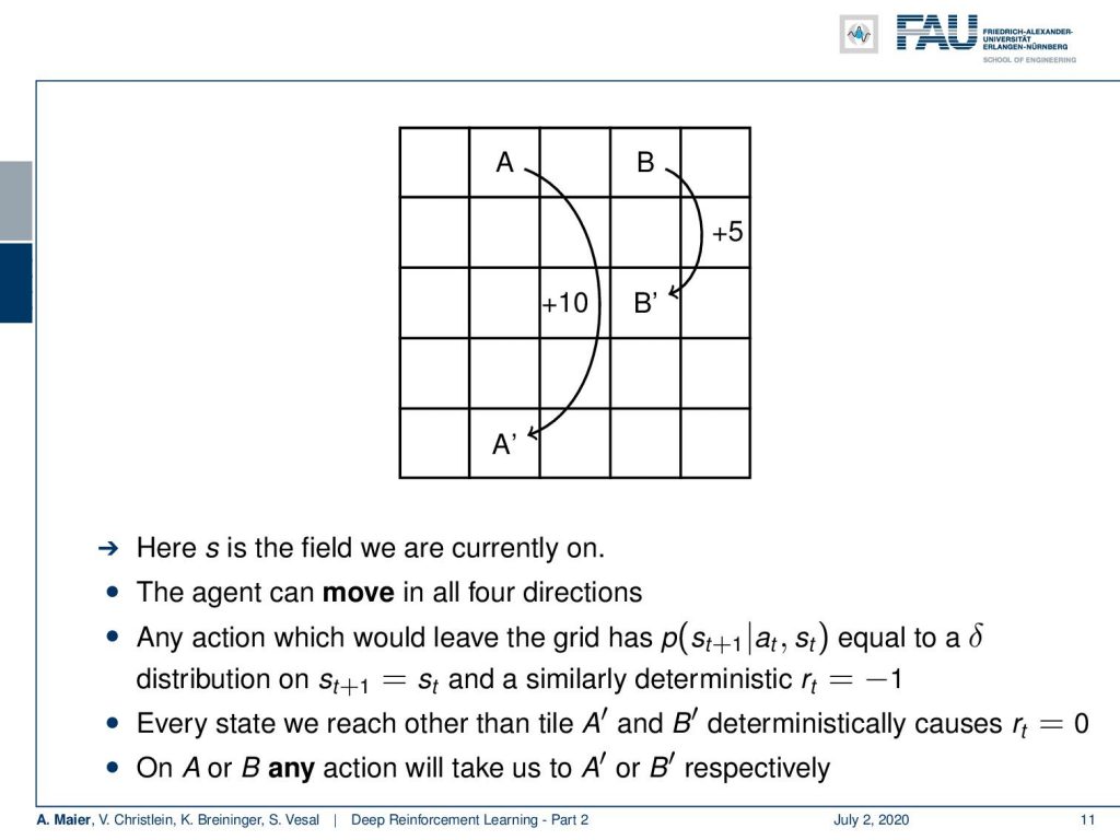
Let’s look at a more simple example rather than controlling robots right away. We will look into a simple game. You see this is a great game. A grid world where we have a couple of squares and our agent then can move across these squares. Of course, the position of the agent is also part of the state. You can formulate this as follows: s is the field that we are currently on. Now, our agent can move in all four directions. So, we can move up, down, left, and right. Any action that would lead the grid has a probability that is equal to a Dirac Delta function that will produce always the previous state. So, you cannot leave the grid. Whenever you try to leave the board, then you are set back to the original position where you tried to leave the board. Furthermore, you get a deterministic reward of -1. So, trying to leave the board is going to be punished with a negative reward. What else? Well, whenever we reach a tile different than A’ and B’, this deterministically causes a reward of 0. So, all of the tiles have no reward. There’s nothing that you gain from moving across the board. The only tiles where you generate a reward is when you arrive at A’ or B’. In order to generate the reward, you have to move to the location A or B. On these locations, you can choose any action it doesn’t matter what you do, but you will be transported to B’ or A’ depending on whether you are on A or B. You there mystically generate a reward of +10 for A and +5 for B. So, this is our game and the game is very simple.
Of course, if you want to play this game or level, you want to generate large rewards. A policy should lead you to the squares A and B and then loop over moving back and forth between A’ and A or B’ and B. So, this would probably be a very good policy to play this game, right? Okay. So now, we somehow have to encode our state and our position. Because we can be on 25 potential different positions, our actions also have to be multiplied by the number of potential positions for this board game. So, let’s have a look at an example policy. The policy is now dependent on the action and the state. The state is more or less the position in this grid and the actions are of course, as we said up, down, left, and right. So now, let’s have a look at the uniform random policy. It can be visualized the way shown here. So, doesn’t matter where we are on the board, we would always choose at equal probability one of the four actions. In this to the grid world example, we can visualize our entire state action space in this simple figure. So, this is very useful for visualization and you can follow this example probably rather well. So, right now with this uniform random policy. Of course, there is no reason to believe that this is a very good policy because we will try to move out of the board, we will occasionally, of course, also hit A and B but it’s not a very good policy.
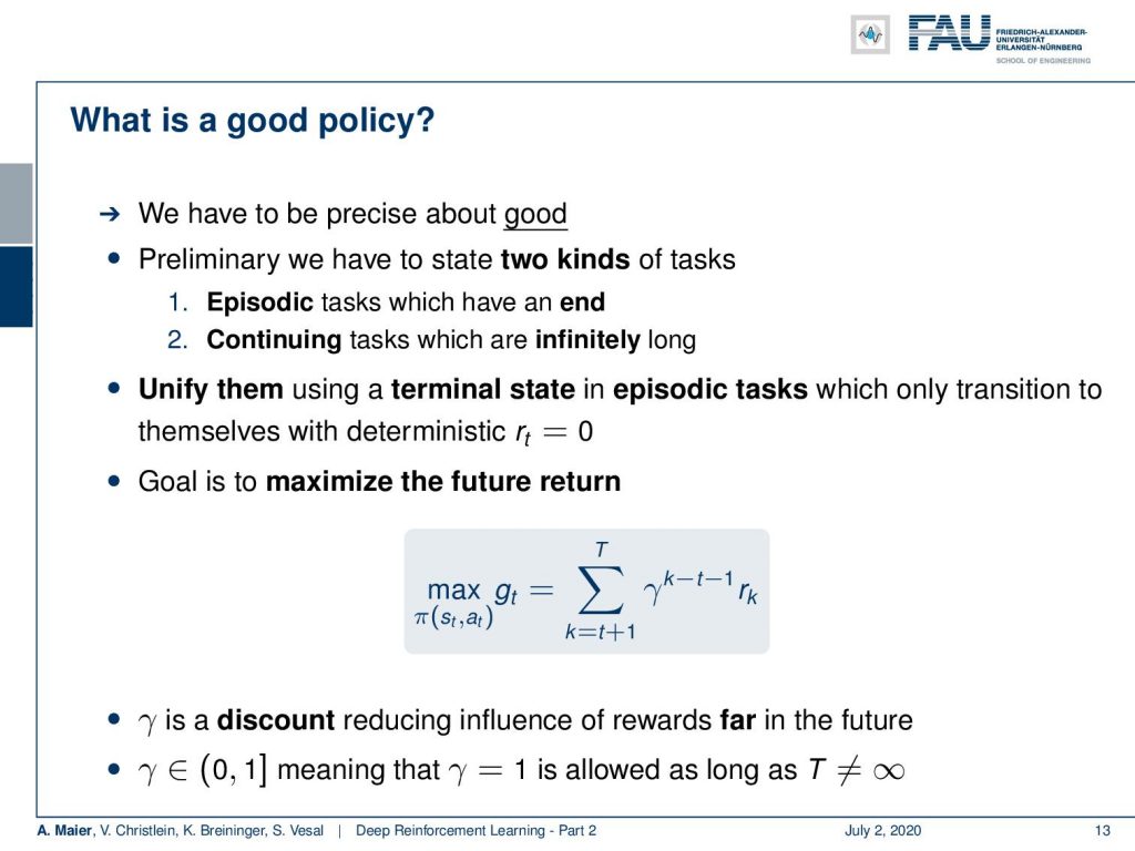
So now, the question is “How can we make better policies?” or “How can we estimate good policies?”. The key question that you have to ask here is you have to ask “What is a good policy?”. So, we have to be very precise about what is good. Essentially, we have to differentiate between two different kinds of tasks. There are episodic tasks that have an end. So they have a beginning and an end like an episode. There are continuing tasks that are infinitely long. So, if you have an infinitely long task, then this is a different situation. Actually, you can unify the two by choosing a terminal state in episodic tasks that only transitions to themselves and produces a deterministic reward of zero. So, you can always make your episodic task into an infinite task by arriving in a final state and this final state continues to produce a zero reward. This, way we don’t have to differentiate between the two any longer. How do we measure what a good policy is? We want to maximize the future return. So, this is very important and in contrast to our multi-armed bandit problem where we simply were essentially averaging or computing the expected value for our rewards, we are now interested in maximizing the future return. So, if you look at this value g subscript t, you can see that this is of course dependent on the policy. So, we seek to maximize our expected future reward with respect to the policy.

We compute it in the following way: So, we start at t + 1 and we iterate all over the sequence until T which is the last element. So, T could also be infinity, if you go towards an infinitely long task. We want to compute the reward that is generated in all of the future time steps until the end of the game. Now, this would be kind of unfair if we don’t take into account how far away our next reward is. So, for example, in the previous game, we will probably try to find the shortest paths to A and B in order to generate a reward. If we would not discount this, so if we have a reward that is high but very far away in the future, it may not be as important to us as a reward that we can generate very quickly. This is why we introduced this discount factor γ here. γ to the power of (k – t – 1) is used to discount rewards that lie far away in the future. If we do so, we implicitly prefer short solutions over long ones. So, we want to get rid of solutions that would randomly move across the board because we want to prefer the shortest paths directly to the reward. This can be accomplished by introducing this discount factor. We see we are now able to describe the goodness or the value of a policy. Now, the problem is, of course, that we want to optimize this expected future reward with respect to the policy. You can’t see even see the policy here in this equation because the policy is the determining factor that produces our reward. One thing that you have to keep in mind is that you choose your discount factor between 0 and 1. The value of 1 is actually allowed as long as your sequence isn’t infinitely long. You can’t have infinity for T in this case. If you have infinitely long sequences then you must choose a discount factor that is lower than 1. Okay. So now, we talked about the very basics, how we can define the Markov decision process, and how we can evaluate the value of a policy.
Of course, what we are still missing and what we talk about next time in deep learning, are the actual implications of this. So, we want to be able to determine good policies and we really want to go into the learning part. So, we want to update the policy in order to make it better in every step. This concept is then called policy iteration. So, I hope you liked this video and you learned the fundamental concept of the Markov decision process and about the evaluation of policies within such a Markov decision process. This is the evaluation of the expected future reward. So, this is a big difference compared to our multi-armed bandit problem, where we’re only looking into the maximum expected reward. Now, we want to take it into account that we want to maximize the reward of the future. Everything, we have done so far it’s not just important, but the foundation for the future steps in order to find a path of winning the game. So thank you very much for listening and hope to see you in the next video! Goodbye!
If you liked this post, you can find more essays here, more educational material on Machine Learning here, or have a look at our Deep LearningLecture. I would also appreciate a follow on YouTube, Twitter, Facebook, or LinkedIn in case you want to be informed about more essays, videos, and research in the future. This article is released under the Creative Commons 4.0 Attribution License and can be reprinted and modified if referenced. If you are interested in generating transcripts from video lectures try AutoBlog.
Links
Link to Sutton’s Reinforcement Learning in its 2018 draft, including Deep Q learning and Alpha Go details
References
[1] David Silver, Aja Huang, Chris J Maddison, et al. “Mastering the game of Go with deep neural networks and tree search”. In: Nature 529.7587 (2016), pp. 484–489.
[2] David Silver, Julian Schrittwieser, Karen Simonyan, et al. “Mastering the game of go without human knowledge”. In: Nature 550.7676 (2017), p. 354.
[3] David Silver, Thomas Hubert, Julian Schrittwieser, et al. “Mastering Chess and Shogi by Self-Play with a General Reinforcement Learning Algorithm”. In: arXiv preprint arXiv:1712.01815 (2017).
[4] Volodymyr Mnih, Koray Kavukcuoglu, David Silver, et al. “Human-level control through deep reinforcement learning”. In: Nature 518.7540 (2015), pp. 529–533.
[5] Martin Müller. “Computer Go”. In: Artificial Intelligence 134.1 (2002), pp. 145–179.
[6] Richard S. Sutton and Andrew G. Barto. Introduction to Reinforcement Learning. 1st. Cambridge, MA, USA: MIT Press, 1998.