
Sequential Decision Making
These are the lecture notes for FAU’s YouTube Lecture “Deep Learning“. This is a full transcript of the lecture video & matching slides. We hope, you enjoy this as much as the videos. Of course, this transcript was created with deep learning techniques largely automatically and only minor manual modifications were performed. Try it yourself! If you spot mistakes, please let us know!
Welcome back to deep learning! So today, we want to discuss the basics of reinforcement learning. We will look into how we can teach a system to play different games and we will start with the very first introduction into sequential decision-making.
So here, I have a couple of slides for you. You see that our topic is reinforcement learning and we want to go ahead and talk about sequential decision-making. Later in this course, we will talk also about reinforcement learning and all the details. We will also look into deep reinforcement learning but today we were only looking to sequential decision-making.
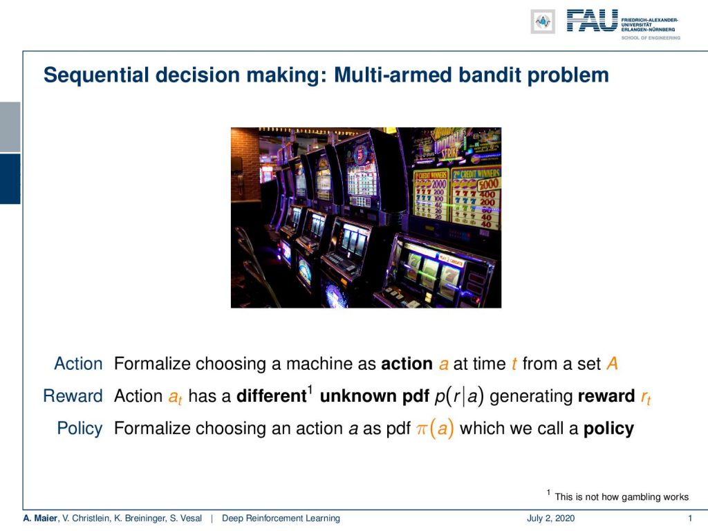
Okay. Sequential decision making! Well, we wanted to play a couple of games. The simplest game that you can potentially think of is that you just pull a couple of levers. If you try to formalize this, then you end up in the so-called multi-armed bandit problem. So, let’s do a couple of definitions: We need some actions and we formalize this as choosing an action a at time t from a set of actions A. So, this is a discrete set of possible actions that we can do. If we choose an action then this has some implications. If you choose a particular action, then you will generate some reward r subscript t. The relation between the action and the reward is probabilistic which means that there is a probably different, yet unknown probability density function that describes the actual relation between the action and the reward. So, if you think of your multi-armed bandit, you have a couple of slot machines, you pull one of the levers, and this generates some reward. But maybe, all of these slot machines are the same. Probably they’re not. So, each arm that you could potentially pull has a different probability of generating some reward. Now, you want to be able to pick an action. In order to do, so we define a so-called policy. The policy is a way of formalizing how to choose an action. It is essentially also a probability density function that describes the likelihood of choosing some action. The policy is essentially the way how we want to influence the game. So, the policy is something that lies in our hands. We can define this policy and of course, we want to make this policy optimal with respect to playing the game.
So, what’s the key element? Well, what do we want to achieve? We want to achieve a maximum reward, In particular, we not just want to have the maximum value for playing the game in every time step. Instead, we want to compute the maximum expected reward over time. So, we produce an estimate of the reward that is going to be produced. We compute a kind of mean value over this because this allows us to then estimate which actions produce what kind of rewards if we play this game over a long time. So, this is a difference to supervised learning because, here, we are not saying do this action or do that action. Instead, we have to determine by our training algorithm which actions to choose. Obviously, we can make mistakes and the aim is then to choose the actions that will over time then produce the maximum expected reward. So, it’s not so important if we lose in one step if we then on average still can generate a high average reward. So, the problem here is, of course, that the expected value of our reward is not known in advance. So, this is the actual problem of reinforcement learning. We want to try to estimate this expected reward and the associated probabilities. So, what we can do is, we can formulate our r subscript t as a one-hot-encoded vector which reflects which action of a has actually caused the reward.
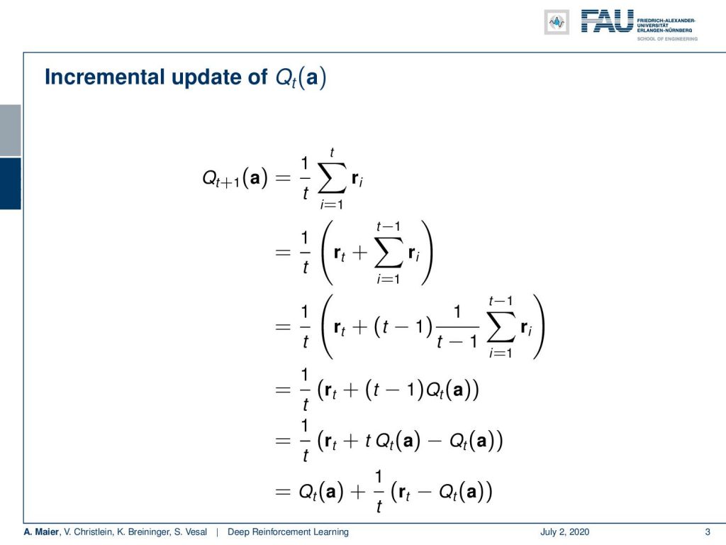
If we do so, we can estimate the probability density function online using an average of the reward. We introduce this as the function Q(a) and this is the so-called action-value function which essentially changes with every new information that we observe. So, how can we do this? Well, there is an incremental way of computing our Q subscript t of a. We can very easily show this. We define Q subscript t as the sum of all the time steps. So, Q subscript t+1 equals to the sum over all the time steps t and the obtained rewards. Of course, you divide by t. Now, we can show that this can be split up. So, we can take out the last element of the sum which is our t and then only have the sum run from 1 to t-1. If we do so, we can then also introduced the term t-1 because if you introduced it here and divide by 1/(t-1), this will cancel out. So, this is a perfectly fine statement. Then, we see that on the right-hand part, we essentially have nothing else then Q subscript t. So, the previous Q subscript t. So, this is something that we have already determined. Then, we can rearrange this a little bit and in the last line, you can see that we can essentially update our Q subscript t+1 as the old Q subscript t plus 1/t times r subscript t minus Q subscript t. So, we can have an incremental formulation of the update of our action-value function. This is very useful because then we don’t have to store all of the rewards but we can do this in an iterative way.
Now, if we go ahead, then we can think about all of the different steps that we have to do in order to train such a system. You end up with something that is called the exploration-exploitation dilemma. So, of course, we want to maximize our reward. We try to choose our policy in a way that we have the maximum reward that we can generate from our action-value function. This would work if you already have a good plan. So, if you already know how things are. So, let’s say you’re looking for the recipe of a pizza and you already have seen a couple of .pizzas that you already like. Then, you can produce the same pizzas again and you know this recipe is good. So, I will get my reward and this would be deterministic if you use the so-called greedy action selection where you always choose the maximum. You always produce the same actions giving the same input. This leads to the problem that we also need to sample our rewards because we don’t know what the best configuration is because we are just exploiting. So, if we only follow the greedy action selection, then we will never make any new observations. We will always produce the same pizza. Maybe there is a much better pizza. Maybe there’s a pizza that we like much better. So, we can only find out if we explore. So every now and then, we have to try a new recipe because otherwise, we don’t know how we should mix the ingredients. Probably, we find a better pizza than the one we already had. This means that on occasions, we have to do moves that will not produce the maximum reward. From not producing a good reward, we can at least learn that this particular move was not a very good one. So, if you train such a system then, in the beginning, you want to focus more on the exploration figuring out which moves are good and which moves are not so good. Then later, you can then exploit it more and more in order to focus on strategies that have worked in certain situations.
So, how can we do that? Well, a very simple form of sampling from actions is the uniform random distribution. So, in the uniform random distribution, you don’t need any knowledge about the system. You just pick actions randomly and you choose them with equal probability. So, you simply select some action and all of the actions are equally likely. The likelihood for every action is one over the cardinality of the set of possible actions. Well, this might be good for exploration, but you probably will make a lot of mistakes. So, there is something that is a little better. This is called the ε-greedy approach. So here, you choose actions given this probability density function. You can see that we choose 1 – ε. So, let’s say ε is 0.1. Then, we choose at 90% probability, the action that maximizes our action-value function, i.e. the action that produces the maximum expected reward. At 10% over n – 1, where n is the number of actions, i.e. for all the other actions, we choose them at this probability. So, you can see that in most cases we will choose, of course, the action that produces the maximum expected reward, but we still can switch to other actions in order to also do some exploration. Of course, the higher you pick your ε the more likely you will be exploring your action space. Then, there are also other variants. For example, you can also use the softmax and introduce some temperature parameter τ. Here, τ can be used in a similar way as we have just been using ε. So here, we find a different formulation where we can use this temperature and then slowly decrease the temperature such that we start looking mostly into the actions that produce the maximum expected reward. So, is this essentially a softer version because here we’d also take into account that other actions may also introduce a different reward. So, if you have two actions that are almost the same in terms of reward, the maximum reward version will, of course, only pick the one that really produces the maximum reward. If you have a reward of 10 and 9, then the softmax function will also split this distribution accordingly.
Well, what have we seen so far? So far, we’ve seen that we can do sequential decision making in a setting that is called the multi-armed bandit problem. We can see that we find a function Q – the so-called action-value function – that is able to describe which expected reward our actions have. Then, we can use this to select our actions. For example, with the greedy action selection, this will always select the action that produces the maximum expected reward. So, we have also seen that if you only do the greedy selection, then we will kind of get stuck because we will never observe certain constellations. If we are missing constellations, we might miss a very good recipe or a very good strategy to win the game or to produce a large reward in that game. So, we need to do exploration as well. Otherwise, we won’t be able to find out what the best strategies are. What we haven’t looked at so far is that our rewards would actually depend on a state of the world. So, in our scenario here, we had everything only connected to the action. The action was the determining factor. But this is a simplification. Of course, a world has a state. This is something, we will consider when we talk about reinforcement learning and Markov Decision Processes. Also, our time didn’t influence rewards. So, in the current constellation, previous actions were completely independent of subsequent actions. This is also a broad simplification which is probably not true in a real application.
This is the reason why we talk next time really on reinforcement learning. In the next video, we will introduce the so-called Markov Decision Process. We will look into what reinforcement learning really is. So, this was only a short teaser about what we can expect when playing games. But in the next video, we will really look into constellation where the world really has a state and where we then also model the dependencies between the different actions. So, it will be a slight bit more complicated. But what you should have learned in this video already that is important is that you find a function that describes the value of a specific action. This is a concept that will come again. The concepts that you should also memorize from here are that you can use the different policies. So, you can have the greedy action selection, the ε-greedy action selection, or the uniform random policy. So, please keep those in mind. They will be important also in future videos when we talk about reinforcement learning. So, thank you very much for listening and hope to see you in the next video. Goodbye!
If you liked this post, you can find more essays here, more educational material on Machine Learning here, or have a look at our Deep LearningLecture. I would also appreciate a follow on YouTube, Twitter, Facebook, or LinkedIn in case you want to be informed about more essays, videos, and research in the future. This article is released under the Creative Commons 4.0 Attribution License and can be reprinted and modified if referenced. If you are interested in generating transcripts from video lectures try AutoBlog.
Links
Link to Sutton’s Reinforcement Learning in its 2018 draft, including Deep Q learning and Alpha Go details
References
[1] David Silver, Aja Huang, Chris J Maddison, et al. “Mastering the game of Go with deep neural networks and tree search”. In: Nature 529.7587 (2016), pp. 484–489.
[2] David Silver, Julian Schrittwieser, Karen Simonyan, et al. “Mastering the game of go without human knowledge”. In: Nature 550.7676 (2017), p. 354.
[3] David Silver, Thomas Hubert, Julian Schrittwieser, et al. “Mastering Chess and Shogi by Self-Play with a General Reinforcement Learning Algorithm”. In: arXiv preprint arXiv:1712.01815 (2017).
[4] Volodymyr Mnih, Koray Kavukcuoglu, David Silver, et al. “Human-level control through deep reinforcement learning”. In: Nature 518.7540 (2015), pp. 529–533.
[5] Martin Müller. “Computer Go”. In: Artificial Intelligence 134.1 (2002), pp. 145–179.
[6] Richard S. Sutton and Andrew G. Barto. Introduction to Reinforcement Learning. 1st. Cambridge, MA, USA: MIT Press, 1998.