A Tribute to Schmidhuber – LSTMs
These are the lecture notes for FAU’s YouTube Lecture “Deep Learning“. This is a full transcript of the lecture video & matching slides. We hope, you enjoy this as much as the videos. Of course, this transcript was created with deep learning techniques largely automatically and only minor manual modifications were performed. If you spot mistakes, please let us know!
Welcome back to deep learning! Today I want to show you one alternative solution to solve this vanishing gradient problem in recurrent neural networks.

You already noticed long temporal contexts are a problem. Therefore, we will talk about long short-term memory units (LSTMs). They have been introduced by a Hochreiter in Schmidhuber and they were published in 1997.
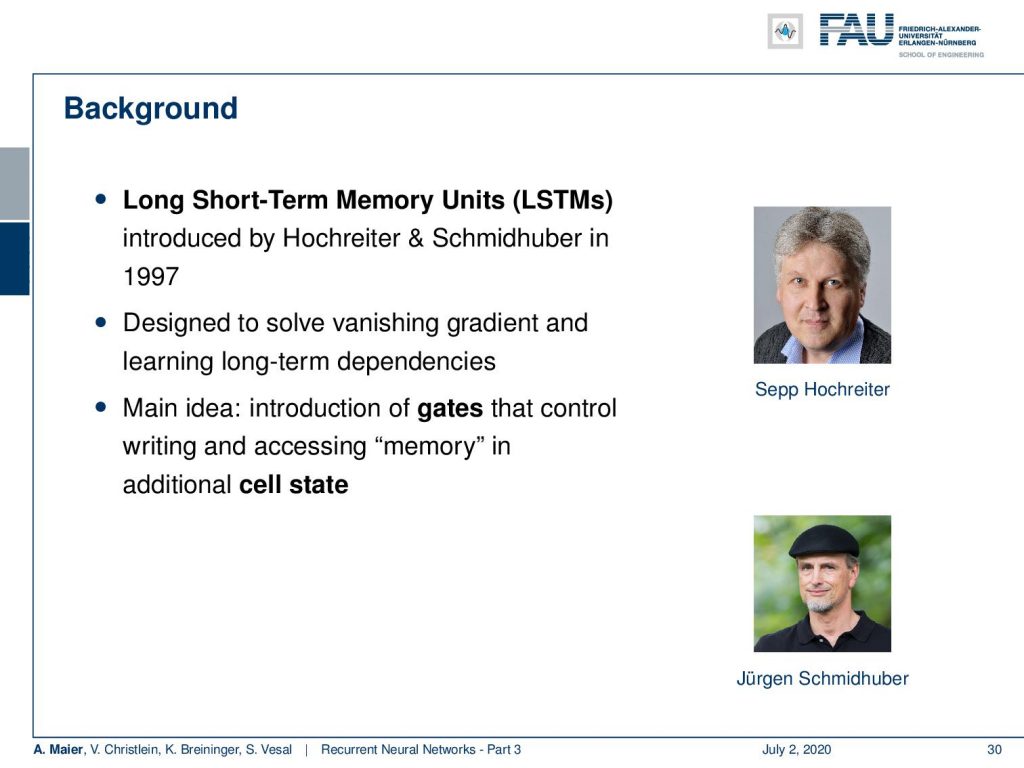
They were designed to solve this vanishing gradient problem in the long term dependencies. The main idea is that you introduce gates that control writing and accessing the memory in additional states.
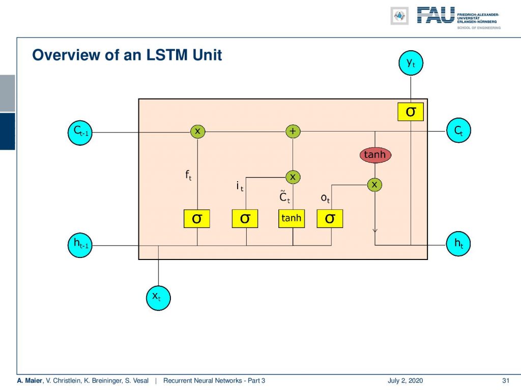
So, let’s have a look into the LSTM unit. You see here, one main feature is that we now have essentially two things that could be considered as a hidden state: We have the cell state C and we have the hidden state h. Again, we have some input x. Then we have quite a few of activation functions. We then combine them and in the end, we produce some output y. This unit is much more complex than what you’ve seen previously in the simple RNNs.
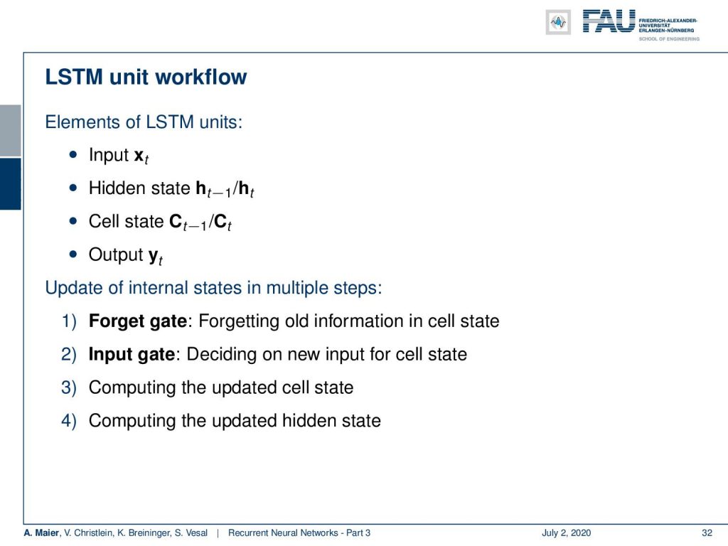
Okay, so what are the main features the LSTM: Given some input x it produces a hidden state h. It also has a cell state C that we will look into a little more detail in the next couple of slides, to produce the output y. Now, we have several gates and the gates essentially are used to control the flow of information. There’s a forget gate and this is used to forget old information in the cell state. Then, we have the input gate and this is essentially deciding new input into the cell state. From this, we then compute the updated cell state and the updated hidden state.
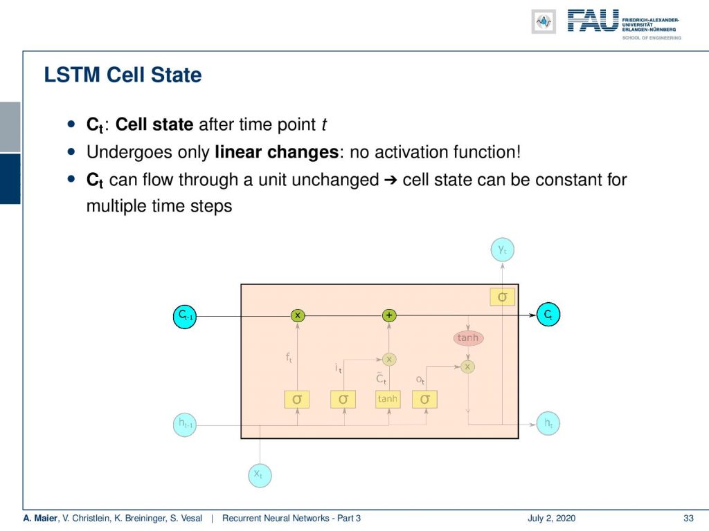
So let’s look into the workflow. We have the cell state after each time point t and the cell state undergoes only linear changes. So there is no activation function. You see there are only one multiplication and one addition on the path of the cell state. So, the cell state can flow through the unit. The cell state can be constant for multiple time steps. Now, we want to operate on the cell state. We do that with several gates and the first one is going to be the forget gate. The key idea here is that we want to forget information from the cell state. In another step, we then want to think about how to actually put new information in the cell state that is going to be used to memorize things.
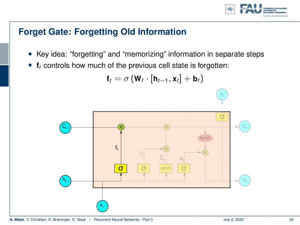
So, the forget gate f controls how much of the previous cell state is forgotten. You can see it is computed by a sigmoid function. So, it’s somewhere between 0 and 1. It’s essentially computed with a matrix multiplication of a concatenation of the hidden state and x plus some bias. This is then multiplied to the cell state. So, we decide which parts of the state vector to forget and which ones to keep.
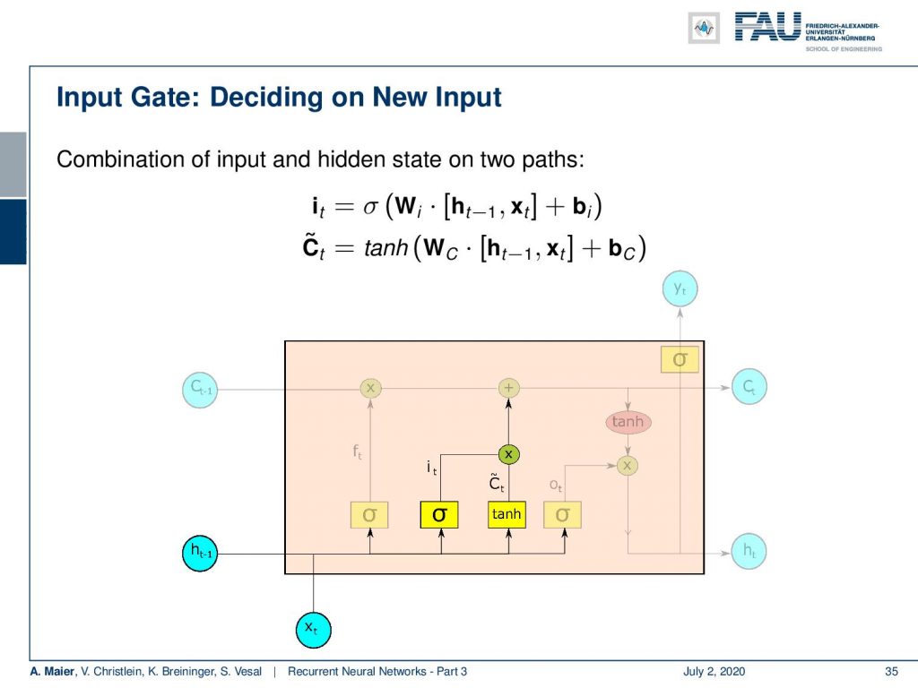
Now, we also need to put in new information. For the new information, we have to somehow decide what information to input into the cell state. So here, we need two activation functions: One that we call I that is also produced by a sigmoid activation function. Again, matrix multiplication of the hidden state concatenated with the input plus some bias and the sigmoid function as non-linearity. Remember, this value is going to be between 0 and 1 so you could argue that it is kind of selecting something. Then, we have some C tilde which is a kind of update state that is produced by the hyperbolic tangent. This then takes as input some weight matrix W subscript c that is multiplied to the concatenation of hidden and input vector plus some bias. So essentially, we have this index that is then multiplied to the intermediate cell stage C tilde. We could say that the hyperbolic tangent is producing some new cell state and then we select via I which of these indices should be added to the current cell state. So, we multiply with I the newly produced C tilde and add it to the cell state C.
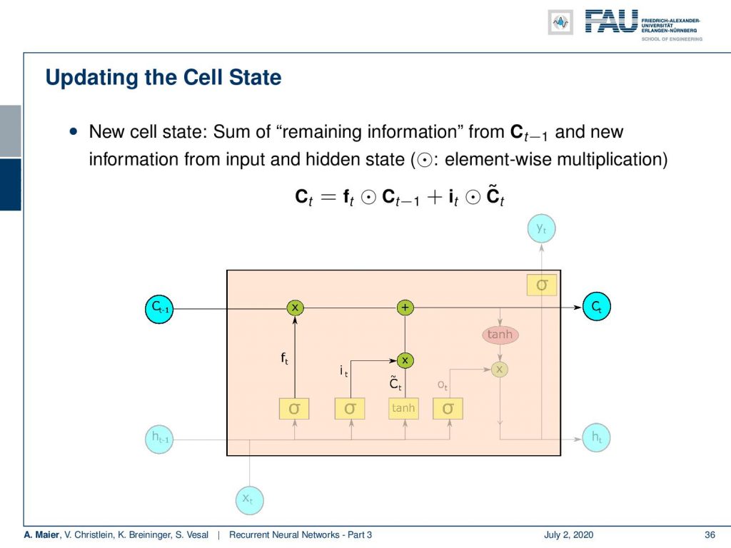
Now, we update as we’ve just seen the complete cell state using a point-wise multiplication with the forget gate of the previous state. Then, we add the elements of the update cell state that have been identified by I with a point-wise multiplication. So, you see the update of the cell state is completely linear only using multiplications and additions.
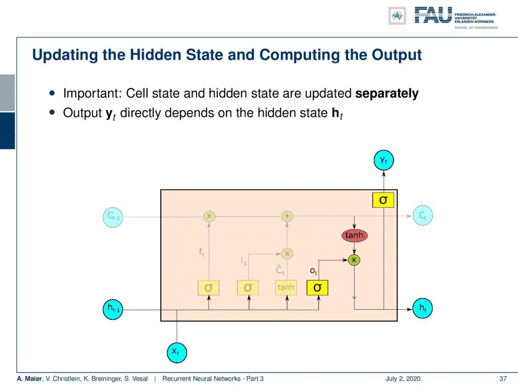
Now, we still have to produce the hidden state and the output. As we have seen in the Elman cell, the output of our network only depends on the hidden state. So, we first update the hidden state by another non-linearity that is then multiplied to a transformation of the cell state. This gives us the new hidden state and from the new hidden state, we produce the output with another non-linearity.
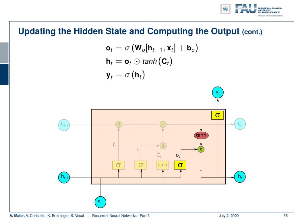
So, you see these are the update equations. We produce some o which is essentially a proposal for the new hidden state by a sigmoid function. Then, we multiply it with the hyperbole tangent that is generated from the cell state in order to select which elements are actually produced. This gives us the new hidden state. The new hidden state we can then pass through another non-linearity in order to produce the output. You can see here, by the way, that for the update of the hidden state and the production of the new output, we omitted the transformation matrices that are of course required. You could interpret each of these nonlinearities in the network essentially as a universal function approximator. So, we still need the linear part, of course, inside here to reduce vanishing gradients.
If you want to train all of this, you can go back and use a very similar recipe as we’ve already seen for the Elman cell. So, you use backpropagation through time in order to update all of the different weight matrices.
Okay. This already brings us to the end of this video. So you’ve seen the long short-term memory cell, the different parts, the different gates, and, of course, this is a very important part of this lecture. So, if you’re preparing for the exam, then I would definitely recommend having a look at how to sketch such a long short-term memory unit. You can see that the LSTM has a lot of advantages. In particular, we can alleviate the problem with the vanishing gradients by the linear transformations in the cell state. By the way, it’s also noteworthy to point out that we somehow include in our long short term memory cell some ideas that we know from computer design. We essentially learn how to manipulate memory cells. We could argue that in the hidden state, we now have the kind of program a kind of finite state machine that then operates on some memory and learns which information to store, which information to delete, and which information to load. So, this is very interesting how these network designs gradually seem to be approaching computer architectures. Of course, there’s much more to say about this. In the next video, we will look into the gated recurrent neural networks which are a kind of simplification of the LSTM cell. You will see that with a slightly slimmer design, we can still get many of the benefits of the LSTM, but much fewer parameters. Ok, so I hope you enjoyed this video and see you next time when we talk about gated recurrent neural networks. Bye-bye!
If you liked this post, you can find more essays here, more educational material on Machine Learning here, or have a look at our Deep LearningLecture. I would also appreciate a follow on YouTube, Twitter, Facebook, or LinkedIn in case you want to be informed about more essays, videos, and research in the future. This article is released under the Creative Commons 4.0 Attribution License and can be reprinted and modified if referenced.
RNN Folk Music
FolkRNN.org
MachineFolkSession.com
The Glass Herry Comment 14128
Links
Character RNNs
CNNs for Machine Translation
Composing Music with RNNs
References
[1] Dzmitry Bahdanau, Kyunghyun Cho, and Yoshua Bengio. “Neural Machine Translation by Jointly Learning to Align and Translate”. In: CoRR abs/1409.0473 (2014). arXiv: 1409.0473.
[2] Yoshua Bengio, Patrice Simard, and Paolo Frasconi. “Learning long-term dependencies with gradient descent is difficult”. In: IEEE transactions on neural networks 5.2 (1994), pp. 157–166.
[3] Junyoung Chung, Caglar Gulcehre, KyungHyun Cho, et al. “Empirical evaluation of gated recurrent neural networks on sequence modeling”. In: arXiv preprint arXiv:1412.3555 (2014).
[4] Douglas Eck and Jürgen Schmidhuber. “Learning the Long-Term Structure of the Blues”. In: Artificial Neural Networks — ICANN 2002. Berlin, Heidelberg: Springer Berlin Heidelberg, 2002, pp. 284–289.
[5] Jeffrey L Elman. “Finding structure in time”. In: Cognitive science 14.2 (1990), pp. 179–211.
[6] Jonas Gehring, Michael Auli, David Grangier, et al. “Convolutional Sequence to Sequence Learning”. In: CoRR abs/1705.03122 (2017). arXiv: 1705.03122.
[7] Alex Graves, Greg Wayne, and Ivo Danihelka. “Neural Turing Machines”. In: CoRR abs/1410.5401 (2014). arXiv: 1410.5401.
[8] Karol Gregor, Ivo Danihelka, Alex Graves, et al. “DRAW: A Recurrent Neural Network For Image Generation”. In: Proceedings of the 32nd International Conference on Machine Learning. Vol. 37. Proceedings of Machine Learning Research. Lille, France: PMLR, July 2015, pp. 1462–1471.
[9] Kyunghyun Cho, Bart Van Merriënboer, Caglar Gulcehre, et al. “Learning phrase representations using RNN encoder-decoder for statistical machine translation”. In: arXiv preprint arXiv:1406.1078 (2014).
[10] J J Hopfield. “Neural networks and physical systems with emergent collective computational abilities”. In: Proceedings of the National Academy of Sciences 79.8 (1982), pp. 2554–2558. eprint: http://www.pnas.org/content/79/8/2554.full.pdf.
[11] W.A. Little. “The existence of persistent states in the brain”. In: Mathematical Biosciences 19.1 (1974), pp. 101–120.
[12] Sepp Hochreiter and Jürgen Schmidhuber. “Long short-term memory”. In: Neural computation 9.8 (1997), pp. 1735–1780.
[13] Volodymyr Mnih, Nicolas Heess, Alex Graves, et al. “Recurrent Models of Visual Attention”. In: CoRR abs/1406.6247 (2014). arXiv: 1406.6247.
[14] Bob Sturm, João Felipe Santos, and Iryna Korshunova. “Folk music style modelling by recurrent neural networks with long short term memory units”. eng. In: 16th International Society for Music Information Retrieval Conference, late-breaking Malaga, Spain, 2015, p. 2.
[15] Sainbayar Sukhbaatar, Arthur Szlam, Jason Weston, et al. “End-to-End Memory Networks”. In: CoRR abs/1503.08895 (2015). arXiv: 1503.08895.
[16] Peter M. Todd. “A Connectionist Approach to Algorithmic Composition”. In: 13 (Dec. 1989).
[17] Ilya Sutskever. “Training recurrent neural networks”. In: University of Toronto, Toronto, Ont., Canada (2013).
[18] Andrej Karpathy. “The unreasonable effectiveness of recurrent neural networks”. In: Andrej Karpathy blog (2015).
[19] Jason Weston, Sumit Chopra, and Antoine Bordes. “Memory Networks”. In: CoRR abs/1410.3916 (2014). arXiv: 1410.3916.