Lecture Notes in Deep Learning: Recurrent Neural Networks – Part 2

Backpropagation through Time

These are the lecture notes for FAU’s YouTube Lecture “Deep Learning“. This is a full transcript of the lecture video & matching slides. We hope, you enjoy this as much as the videos. Of course, this transcript was created with deep learning techniques largely automatically and only minor manual modifications were performed. If you spot mistakes, please let us know!

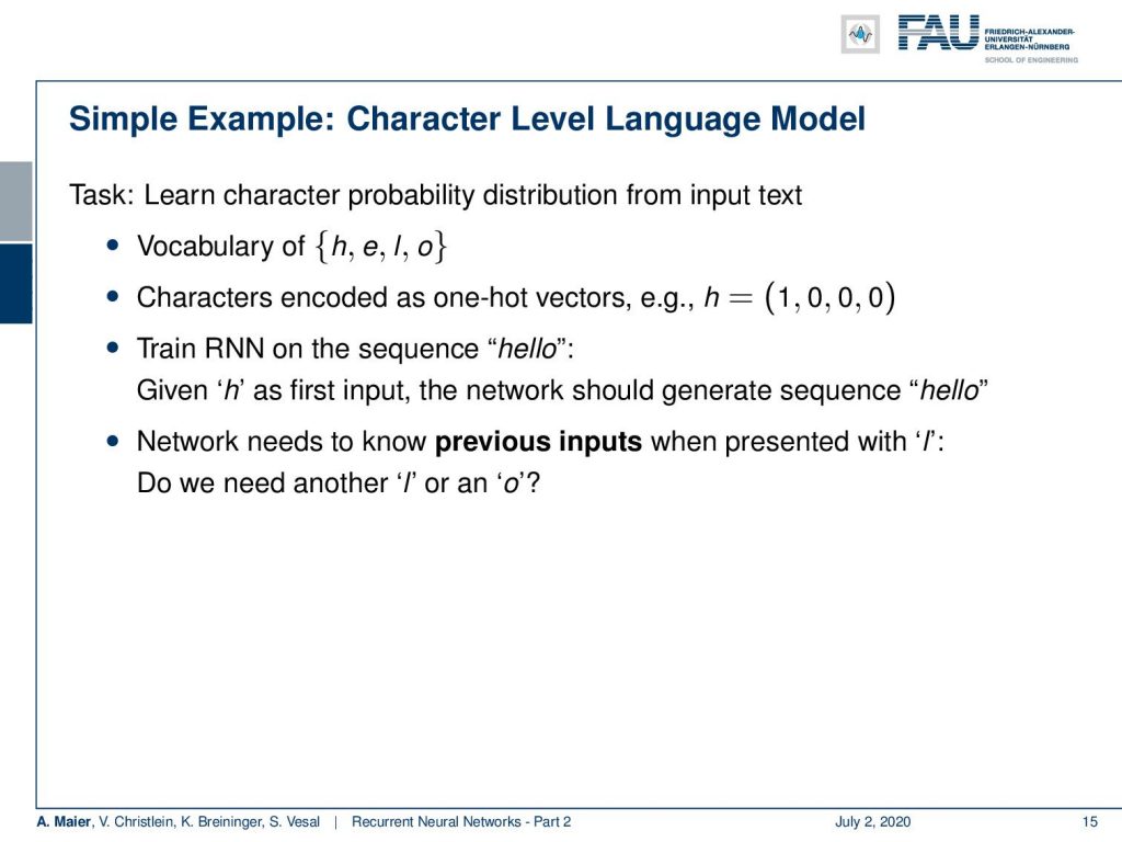
Welcome back to deep learning! Today we want to talk a little bit more about recurrent neural networks and in particular look into the training procedure. So how does our RNN training work? Let’s look at a simple example and we start with a character level language model. So, we want to learn a character probability distribution from an input text and our vocabulary is going to be very easy. It’s gonna be the letters h, e, l, and o. We’ll encode them as one-hot vectors which then gives us for example for h the vector (1 0 0 0)ᵀ. Now, we can go ahead and train our RNN on the sequence “hello” and we should learn that given “h” as the first input, the network should generate the sequence “hello”. Now, the network needs to know previous inputs when presented with an l because it needs to know whether it needs to generate an l or an o. It’s the same input but two different outputs. So, you have to know the context.

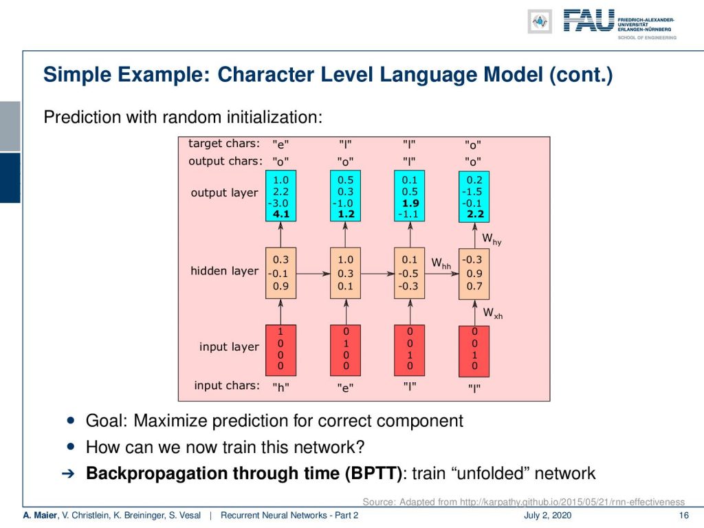
Let’s look at this example and here you can already see how the decoding takes place. So, we put in essentially on the input layer again as one-hot encoded vectors the inputs. Then, we produce the hidden state h subscript t with the matrices that we’ve seen previously and produce outputs and you can see. Now, we feed in the different letters and this then produces some outputs that can then be mapped via one-hot encoding back to letters. So, this gives us essentially the possibility to run over the entire sequence and produce the desired outputs. Now, for the training, the problem is how can we determine all of these weights? Of course, we want to maximize these weights with respect to predicting the correct component.

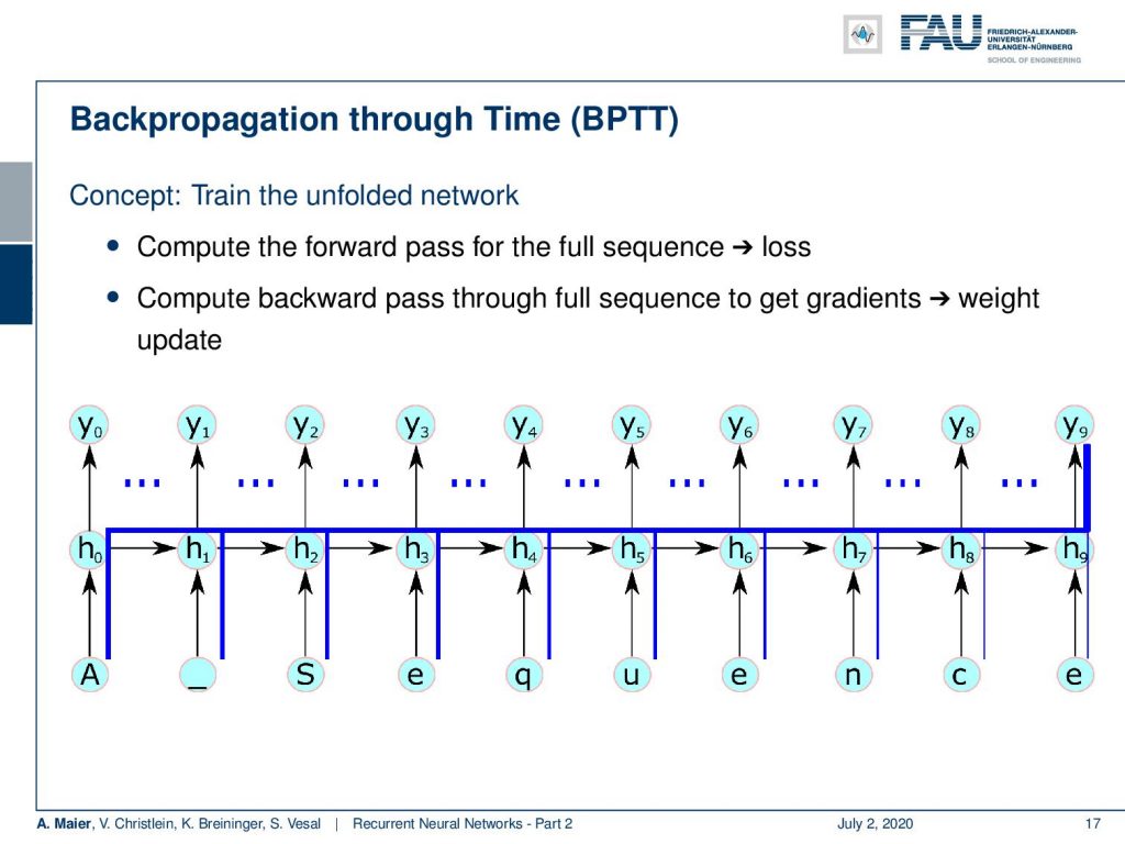
This all can be achieved with the backpropagation through time algorithm. The idea is we train on the unfolded network. So here’s a short sketch on how to do this. The idea is that we unfold the network. So, we compute the forward path for the full sequence and then we can apply the loss. So, we essentially then backpropagate over the entire sequence such that even things that happen in the very last state can have an influence on the very beginning. So, we compute the backward pass through the full sequence to get the gradients and the weight update. So, for one update with backpropagation through time, I have to unroll this complete network that then is generated by the input sequence. Then, I can compare the output that was created with the desired output and compute the update.

So, let’s look at this in a little bit more detail. The forward pass is, of course, just the computation of the hidden states and the output. So, we know that we have some input sequence that is x subscript 1 to x subscript T, where T is the sequence length. Now, I just repeat update our u subscript t which is the linear part before the respective activation function. Then, we compute the activation function to get our new hidden state then we compute the o subscript t which is essentially the linear part before the sigmoid function. Then, we apply the sigmoid to produce the y hat that is essentially the output of our network.

If we do so, then we can unroll the entire network and produce all of the respective information that we need to then actually compute the update for the weights.

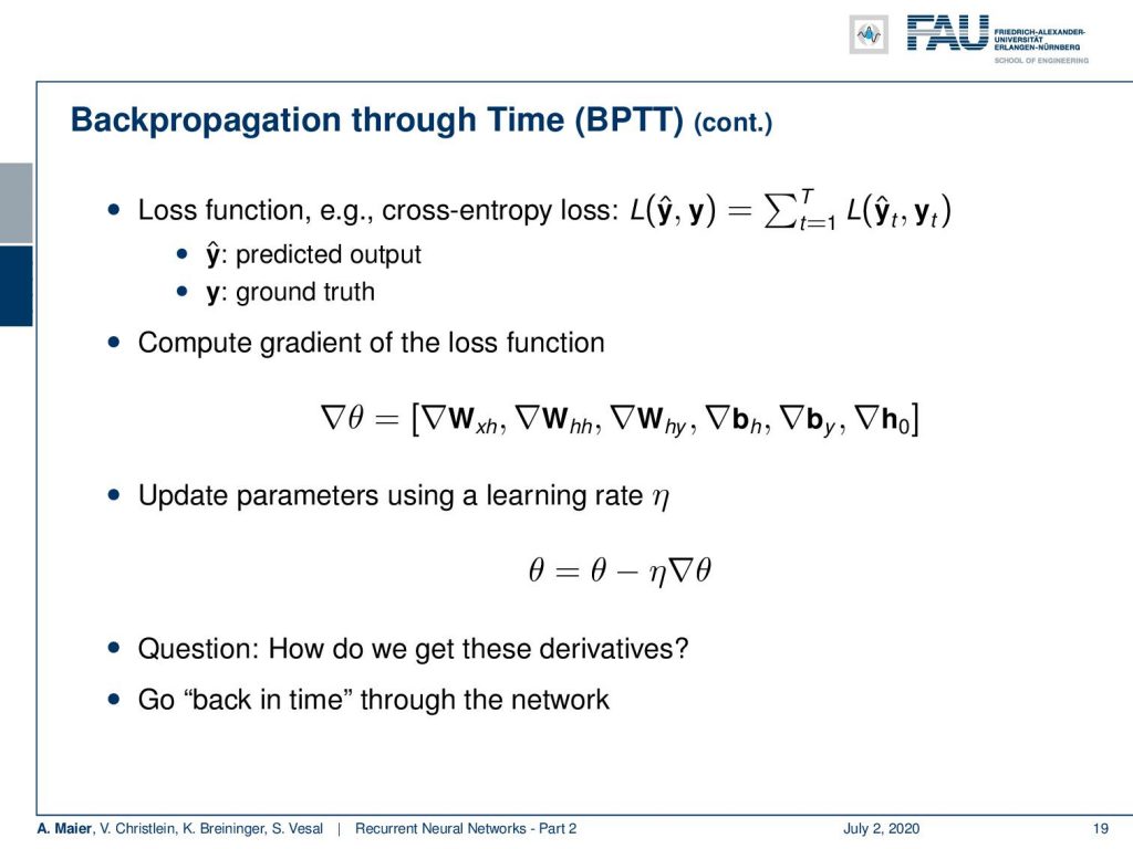
Now the backpropagation through time then essentially produces a loss function. Now, the loss function is summing up essentially the losses that we already know from our previous lectures, but we sum it up over the actual observations at every time t. So, we can, for example, take cross-entropy, then we compare the predicted output with the ground truth and compute the gradient of the loss function in a similar way as we already know it. We want to get the parameter update for our parameter vector θ that is composed of those three matrices, the two bias vectors, and the vector h. So, the update of the parameters can then also be done using a learning rate in a very similar way as we have been doing this throughout the entire class. Now, the question is, of course, how do we get those derivatives and the idea is now to go back in time through the entire network.

So what do we do? Well, we start at time t equals T and then iteratively compute the gradients for T up to 1. So just keep in mind that our y hat was produced by the sigma of o subscript t which is composed of those two matrices. So, if we want to compute the partial derivative with respect to o subscript t, then we need the derivative of the sigmoid functions of o subscript t times the partial derivative of the loss function with respect to y hat subscript t. Now, you can see that the gradient with respect to W subscript hy is going to be given as the gradient of o subscript t times h subscript t transpose. The gradient with respect to the bias is going to be given simply as the gradient of o subscript t. So, the gradient h subscript t now depends on two elements: the hidden state that is influenced by o subscript t and the next hidden state h subscript t+1. So, we can get the gradient of h subscript t as the partial derivative of h subscript t+1 with respect to h subscript t transpose times the gradient of h subscript t+1. Then, we still have to add the partial derivative of o subscript t with respect to h subscript t transposed times the gradient of o subscript t. This can then be expressed as the weight matrix W subscript hh transpose times the tangens hyperbolicus derivative of W subscript hh times h subscript t plus W subscript xh times x subscript t+1 plus the bias h multiplied with the gradient of h subscript t+1 plus W subscript hy transposed times the gradient of o subscript t. So, you can see that we can also implement this gradient with respect to matrices. Now, you already have all the updates for the hidden state.

Now, we also want to compute the updates for the other weight matrices. So, let’s see how this is possible. We now have established essentially the way of computing the derivative with respect to our h subscript t. So, now we can already propagate through time. So for each t, we essentially get one element in the sum and because we can compute the gradient h subscript t, we can now get the remaining gradients. In order to compute h subscript t, you see that we need the tanh of u subscript t which then contains the remaining weight matrices. So we essentially get the derivative respect to the two missing matrices and the bias. By using the gradient h subscript t times the tangens hyperbolicus derivative of u subscript t. Then, depending on which matrix you want to update, it’s gonna be h subscript t-1 transpose, or x subscript t transpose. For the bias, you don’t need to multiply with anything extra. So, these are essentially the ingredients that you need in order to compute the remaining updates. What we see now is that we can compute the gradients, but they are dependent on t. Now, the question is how do we get the gradient for the sequence. What we see is that the network that emerges in the unrolled state is essentially a network of shared weights. This means that we can update simply by the sum over all time steps. So this then allows us to compute essentially all the updates for the weights and every time t. Then, the final gradient update is gonna be the sum of all those gradient steps. Ok, so we’ve seen how to compute all these steps and yes: It’s maybe five lines of pseudocode, right?

Well, there are some problems with normal backpropagation through time. You need to unroll the entire sequence and for long sequences and complex networks, this can mean a lot of memory consumption. A single parameter update is very expensive. So, you could do a splitting approach like the naive approach that we’re suggesting here, but if you would just split the sequence into batches and then start again initializing the hidden state, then you can probably train but you lose dependencies over long periods of time. In this example, the first input can never be connected to the last output here. So, we need a better idea of how to proceed and save memory and, of course, there’s an approach to do so. This is called the truncated backpropagation through time algorithm.

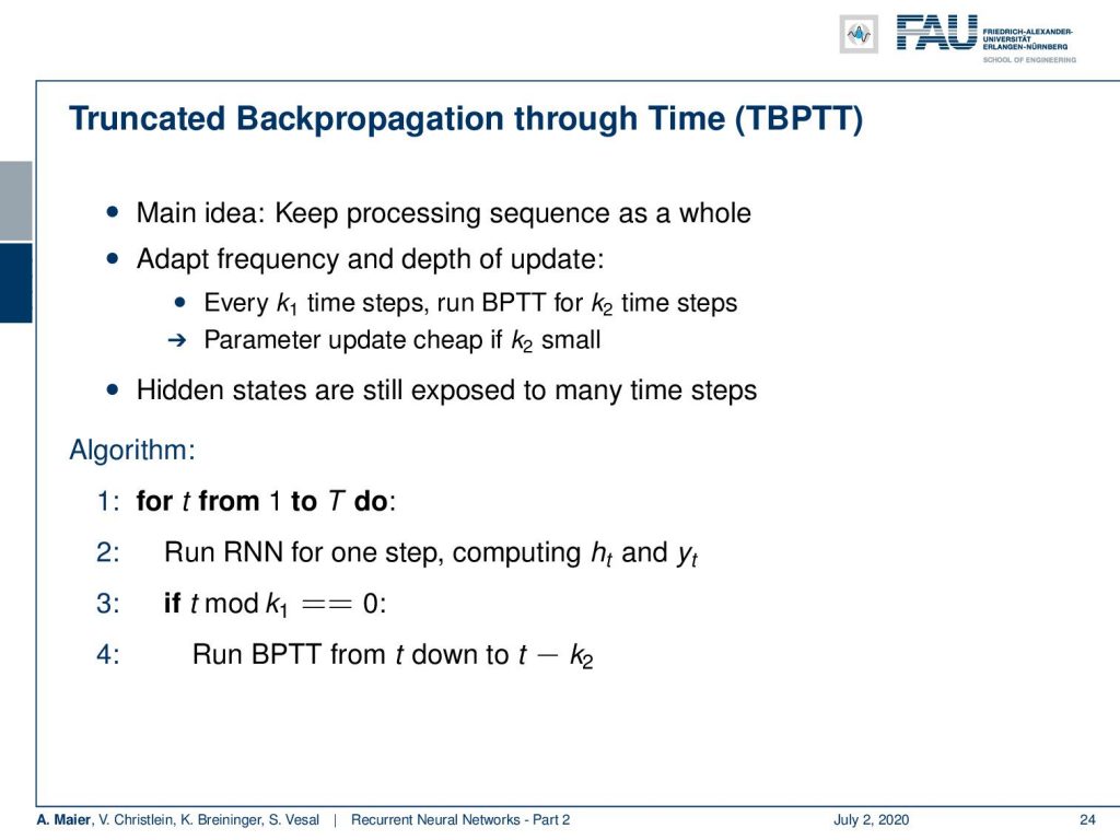
Now, the truncated backpropagation through time algorithm keeps the processing of the sequence as a whole, but it adapts the frequency and depth of the updates. So every k₁ time steps, you run a backpropagation through time for k₂ time steps and the parameter update is gonna be cheap if k₂ is small. The hidden states are still exposed to many time steps as you will see in the following. So, the idea is for time t from 1 to T to run our RNN for one step computing h subscript t and y subscript t and then if we are at the k₁ step, then we run backpropagation through time from T down to t minus k₂.

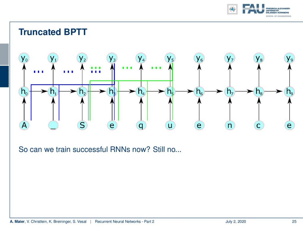
This then emerges in the following setup: What you can see here is that we essentially step over 4 time steps. If we are in the fourth time step, then we can backpropagate through time until the beginning of the sequence. Once we did that, we process ahead and we always keep the hidden state. We don’t discard it. So, we can model this interaction. So, does this solve all of our problems? Well, no because if we have a very long temporal context, it will not be able to update. So let’s say, the first element is responsible for changing something in the last element of your sequence, then you see they will never be connected. So, we are not able to learn this long temporal context anymore. This is a huge problem with long term dependency and basic RNNs.

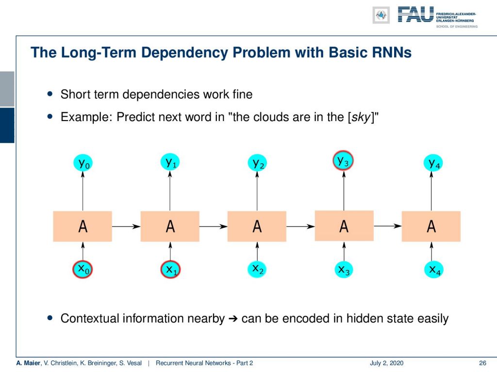
So, let’s say you have this long term dependency. You want to predict the next word in “the clouds are in the sky”. You can see that the clouds are probably a relevant context for this. Here, the context information is rather nearby. So, we can encode it in the hidden state rather easily. Now, if we have very long sequences, then it will be much harder because we have to backpropagate over so many steps. You have seen also that we had these problems in deep networks where we had the vanishing gradient problem. We were not able to find updates that connect parts of networks that are very far apart from each other.

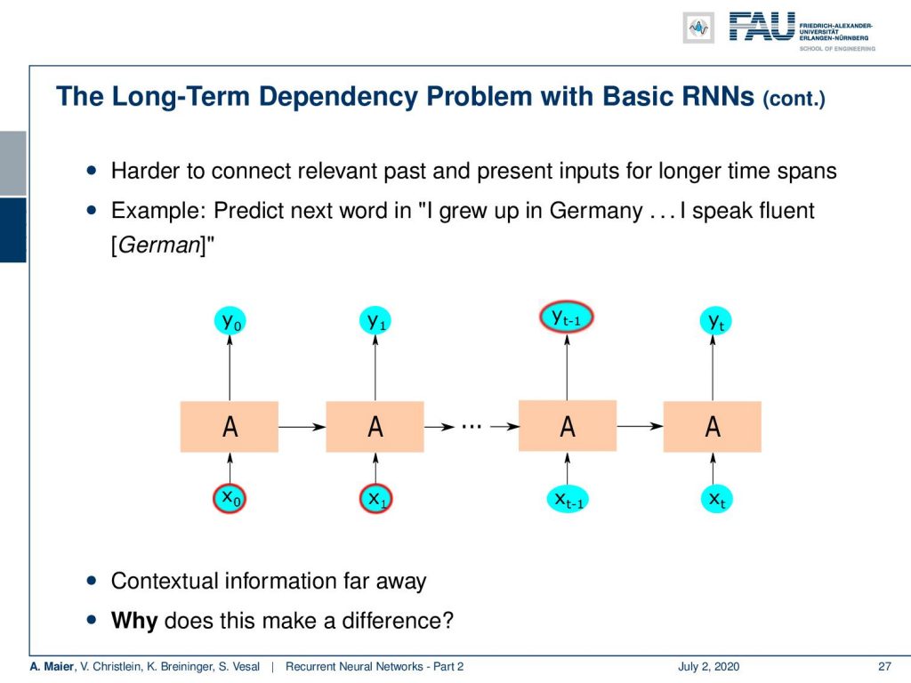
You can see here that if we have this example: a sentence like “I grew up in Germany” and then say something else and “I speak fluent”, it’s probably German. I have to be able to remember that “I grew up in Germany”. So, the contextual information is far away and this makes a difference because we have to propagate through many layers.

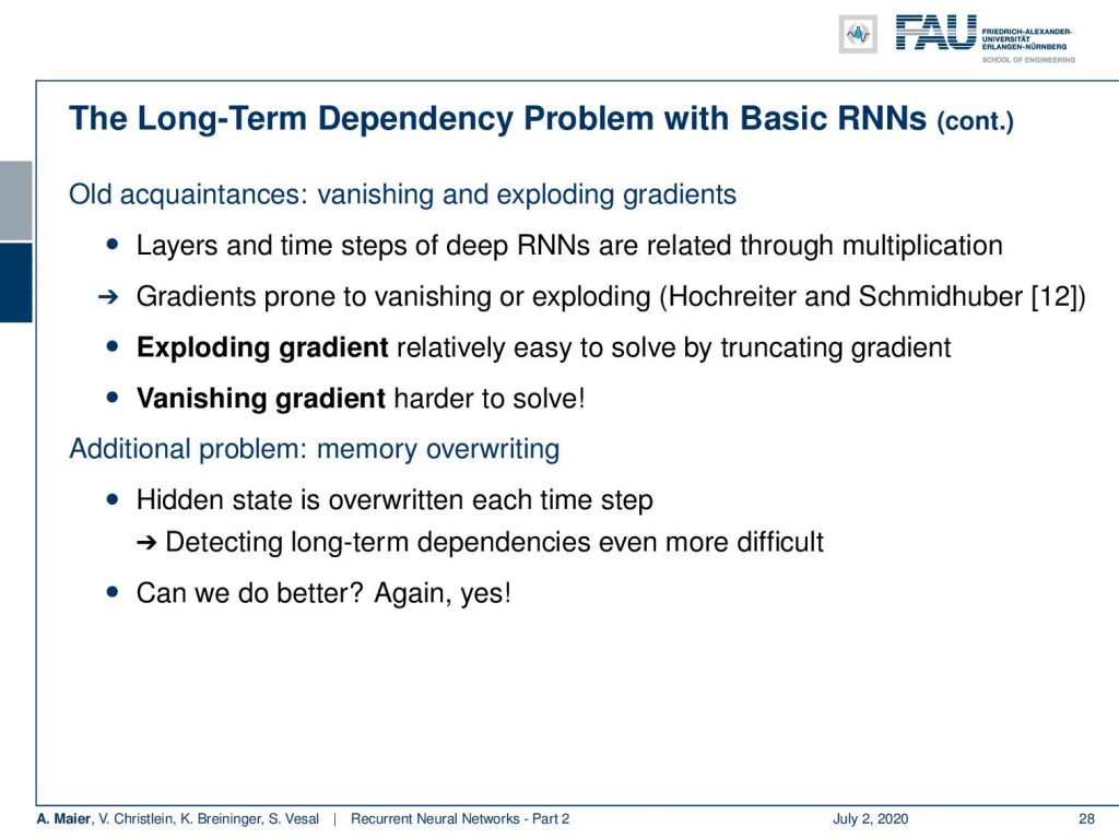
This means that we have to multiply with each other. You can see that those gradients are prone to vanishing and exploding as by the way identified by Hochreiter and Schmidhuber in [12]. Now, you still have this problem that you could have an exploding gradient. Well, you can truncate the gradient but the vanishing gradient is much harder to solve. There’s another problem the memory overwriting because the hidden state is overwritten in each time step. So detecting long-term dependencies will be even more difficult if you don’t have enough space in your hidden state vector. This is also a problem that may occur in your recurrent neural network. So, can we do better than this? The answer is again: yes.

This is something we will discuss in the next video, where we then talk about long short-term memory units and the contributions that were done by Hochreiter and Schmidhuber.

So thank you very much for listening to this video and hope to see you in the next one. Thank you and goodbye!

If you liked this post, you can find more essays here, more educational material on Machine Learning here, or have a look at our Deep LearningLecture. I would also appreciate a follow on YouTube, Twitter, Facebook, or LinkedIn in case you want to be informed about more essays, videos, and research in the future. This article is released under the Creative Commons 4.0 Attribution License and can be reprinted and modified if referenced.

RNN Folk Music

FolkRNN.org
MachineFolkSession.com
The Glass Herry Comment 14128

Links

Character RNNs
CNNs for Machine Translation
Composing Music with RNNs

References

[1] Dzmitry Bahdanau, Kyunghyun Cho, and Yoshua Bengio. “Neural Machine Translation by Jointly Learning to Align and Translate”. In: CoRR abs/1409.0473 (2014). arXiv: 1409.0473.
[2] Yoshua Bengio, Patrice Simard, and Paolo Frasconi. “Learning long-term dependencies with gradient descent is difficult”. In: IEEE transactions on neural networks 5.2 (1994), pp. 157–166.
[3] Junyoung Chung, Caglar Gulcehre, KyungHyun Cho, et al. “Empirical evaluation of gated recurrent neural networks on sequence modeling”. In: arXiv preprint arXiv:1412.3555 (2014).
[4] Douglas Eck and Jürgen Schmidhuber. “Learning the Long-Term Structure of the Blues”. In: Artificial Neural Networks — ICANN 2002. Berlin, Heidelberg: Springer Berlin Heidelberg, 2002, pp. 284–289.
[5] Jeffrey L Elman. “Finding structure in time”. In: Cognitive science 14.2 (1990), pp. 179–211.
[6] Jonas Gehring, Michael Auli, David Grangier, et al. “Convolutional Sequence to Sequence Learning”. In: CoRR abs/1705.03122 (2017). arXiv: 1705.03122.
[7] Alex Graves, Greg Wayne, and Ivo Danihelka. “Neural Turing Machines”. In: CoRR abs/1410.5401 (2014). arXiv: 1410.5401.
[8] Karol Gregor, Ivo Danihelka, Alex Graves, et al. “DRAW: A Recurrent Neural Network For Image Generation”. In: Proceedings of the 32nd International Conference on Machine Learning. Vol. 37. Proceedings of Machine Learning Research. Lille, France: PMLR, July 2015, pp. 1462–1471.
[9] Kyunghyun Cho, Bart Van Merriënboer, Caglar Gulcehre, et al. “Learning phrase representations using RNN encoder-decoder for statistical machine translation”. In: arXiv preprint arXiv:1406.1078 (2014).
[10] J J Hopfield. “Neural networks and physical systems with emergent collective computational abilities”. In: Proceedings of the National Academy of Sciences 79.8 (1982), pp. 2554–2558. eprint: http://www.pnas.org/content/79/8/2554.full.pdf.
[11] W.A. Little. “The existence of persistent states in the brain”. In: Mathematical Biosciences 19.1 (1974), pp. 101–120.
[12] Sepp Hochreiter and Jürgen Schmidhuber. “Long short-term memory”. In: Neural computation 9.8 (1997), pp. 1735–1780.
[13] Volodymyr Mnih, Nicolas Heess, Alex Graves, et al. “Recurrent Models of Visual Attention”. In: CoRR abs/1406.6247 (2014). arXiv: 1406.6247.
[14] Bob Sturm, João Felipe Santos, and Iryna Korshunova. “Folk music style modelling by recurrent neural networks with long short term memory units”. eng. In: 16th International Society for Music Information Retrieval Conference, late-breaking Malaga, Spain, 2015, p. 2.
[15] Sainbayar Sukhbaatar, Arthur Szlam, Jason Weston, et al. “End-to-End Memory Networks”. In: CoRR abs/1503.08895 (2015). arXiv: 1503.08895.
[16] Peter M. Todd. “A Connectionist Approach to Algorithmic Composition”. In: 13 (Dec. 1989).
[17] Ilya Sutskever. “Training recurrent neural networks”. In: University of Toronto, Toronto, Ont., Canada (2013).
[18] Andrej Karpathy. “The unreasonable effectiveness of recurrent neural networks”. In: Andrej Karpathy blog (2015).
[19] Jason Weston, Sumit Chopra, and Antoine Bordes. “Memory Networks”. In: CoRR abs/1410.3916 (2014). arXiv: 1410.3916.

Category: Lecture Notes in Deep Learning