Lecture Notes in Deep Learning: Known Operator Learning – Part 2

Boundaries on Learning

These are the lecture notes for FAU’s YouTube Lecture “Deep Learning“. This is a full transcript of the lecture video & matching slides. We hope, you enjoy this as much as the videos. Of course, this transcript was created with deep learning techniques largely automatically and only minor manual modifications were performed. Try it yourself! If you spot mistakes, please let us know!

Welcome back to deep learning! So, today I want to continue to talk to you about known operators. In particular, I want to show you how to embed these known operations into the network and what kind of theoretical implications are created by this. So, the key phrase will be “Let’s not re-invent the wheel.”

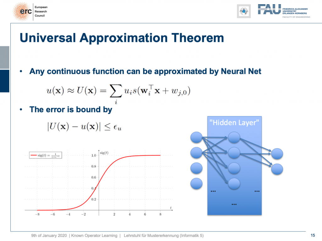
We go back all the way to our universal approximation theorem. The universal approximation theorem told us that we can find a one hidden layer representation that approximates any continuous function u(x) with an approximation U(x) and it is supposed to be very close. It’s computed as a superposition linear combination of sigmoid functions. We know that there is a bound ε subscript u. ε subscript u tells us the maximum difference between the original function and the approximated function and this is exactly one hidden layer in your network.

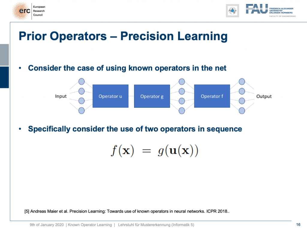
Well, this is nice but we are not really interested in one-hidden-layer neural networks, right? We would be interested in an approach that we coined precision learning. So here, the idea is that we want to mix approximators with known operations and embed them into the network. Specifically, the configuration that I have here is a little big for theoretical analysis. So, let’s go to a little simpler problem. Here, we just say okay we have a two-layer network where we have a transform from x using u(x). So, this is a vector to vector transform. This is why it’s in boldface. Then, we have some transform g(x). It takes the output of u(x) and produces a scalar value. This is then essentially the definition of f(x). So here, we know that f(x) is composed of two different functions. So, this is already the first postulate here that we need in order to look into known operator learning.

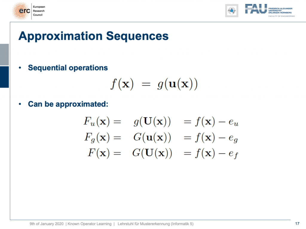
We now want to approximate composite functions. If I look at f, we can see that there are essentially three choices of how we can approximate it. We can approximate only U(x). Then, this would give us F subscript u. We could approximate only G(x). This would result in F subscript g, or we could approximate both of them. That is then G(U(x)) using both of our approximations. Now, with any of these approximations, I’m introducing an error. The error can be described as e subscript u, if I approximate U(x) and e subscript g, if I approximate G(x), and e subscript f, if I approximate both.

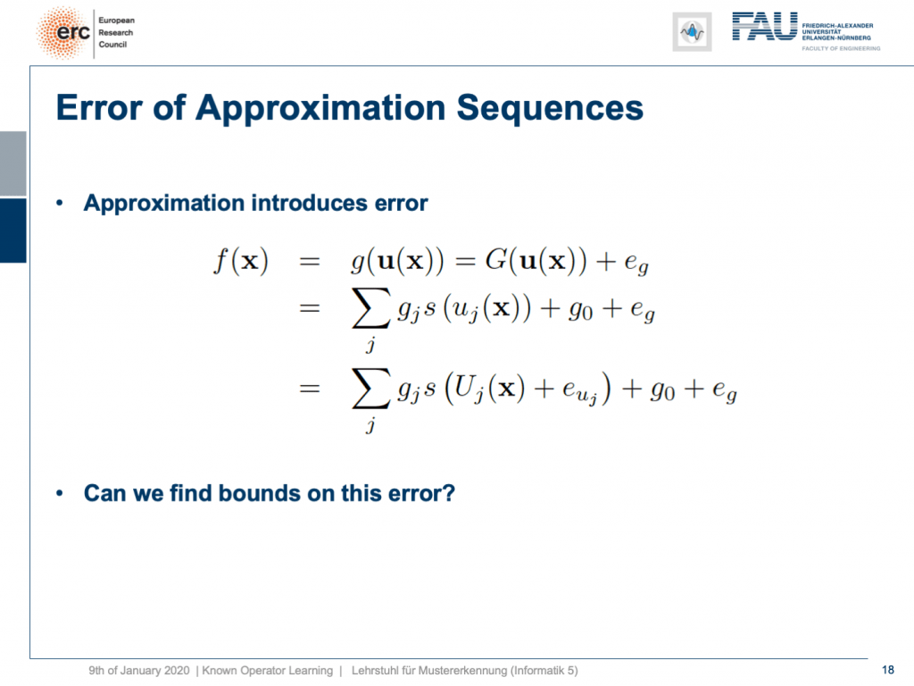
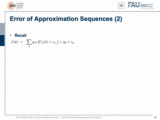
So, let’s look into the math and see what we can do with those definitions. Well, of course, we can start with f(x). We use the definition of f(x). Then, the definition gives us g(u(x)). We can start approximating G(x). Now, if you’re approximate it, we introduce some error e subscript g. The error has to be added back. This is then shown here in the next line. We can see we can also use the definition of G(x) that is a linear combination of sigmoid functions. Here, we then use component-wise the original function u subscript j, because it is a vectorial function. Of course, we have the different weights g subscript j, the bias g subscript 0, and the error that we introduced by approximating g(x). So, we can also now approximate u(x) component-wise. Then, we introduce an approximation and the approximation, of course, also introduces an error. So, this is nice, but we kind of get stuck here because the error of the approximation of u(x) is inside of the sigmoid function. All the other errors are outside. So, what can we do about this? Well, least we can look into error bounds.

So, let’s have a look at our bounds. The key idea here is that we use the property of the sigmoid function that it has a Lipschitz bound. So, there is a maximum slope that occurs in this function and that is denoted by l subscript s meaning that if I’m at the position x and I move to a direction e, then I can always find an upper bound by taking the magnitude of e times the highest slope that occurs in the function plus the original function value. So, it’s a linear extrapolation and you can see this in this animation. We essentially have the two white cones that always will be above or below the function. Obviously, we can also construct a lower bound using the Lipschitz property. Well, now what can we do with this? We can now go ahead and use it for our purposes but we just run into the next problem. Our Lipschitz bound here doesn’t hold for linear combinations. So, you see that we are actually interested in multiplying this with some weight g subscript j. As soon as I take a negative g subscript j, then this would essentially mean that our inequality flips. So, this is not cool but we can find an alternative formulation like the bottom one. So, we simply have to use an absolute value when we multiply with the Lipschitz constant in order to remain above the function all the time. Running through the proof here is kind of tedious. This is why I brought you the two images here. So, we reformulated this and we took all the terms on the right-hand side, subtracted them, and move them to the left-hand side which means that all of these terms need to be in combination lower than zero. If you do that for positive and negative g subscript j, you can see in the two plots that independent of the choice of e and x, I’m always below zero. You can also go to the original reference if you’re interested in the formal proof for this [5].

So now, let’s use this inequality. We can see now that we can finally get our e subscript uj out of the bracket snd out of the sigmoid function. We get an upper bound by using this kind of approximation. Then, we can see if we arrange the terms correctly that the first couple of terms are simply the definition of F(x). So, this is the approximation using G(x) and U(x). This then can be simplified to just write down F(x). This, plus the sum over the components of G(x) times the Lipschitz times the absolute value of the error plus the error that we introduced by G. Now, we can essentially subtract F(x) and if we do so, we can see that f(x) – F(x) is nothing else than the error introduced when doing this approximation. So, this is simply e subscript f. So, we have an upper bound for the error in e subscript f that is composed as the sum on the right-hand side. We can still replace the e subscript g by ε subscript g which is the upper bound to e subscript g. It’s still an upper bound to e subscript f. Now, these are all upper bounds.

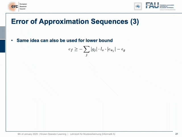
The same idea can also be used to get a lower bound. You see that then we have this negative sum. This is always a lower bound. Now, if we have the upper and the lower bound, then we can see that the magnitude of e subscript f is bound by the sum over the components g subscript j times the Lipschitz constant times the error plus ε subscript g. This is interesting because here we see that this is essentially the error of U(x) amplified with the structure of G(x) plus the error introduced by G. So, if we know u(x) the error u cancels out, and if we know g(x) the error g cancels out, and of course, if we know both, there is no error because there’s nothing that we have to learn.

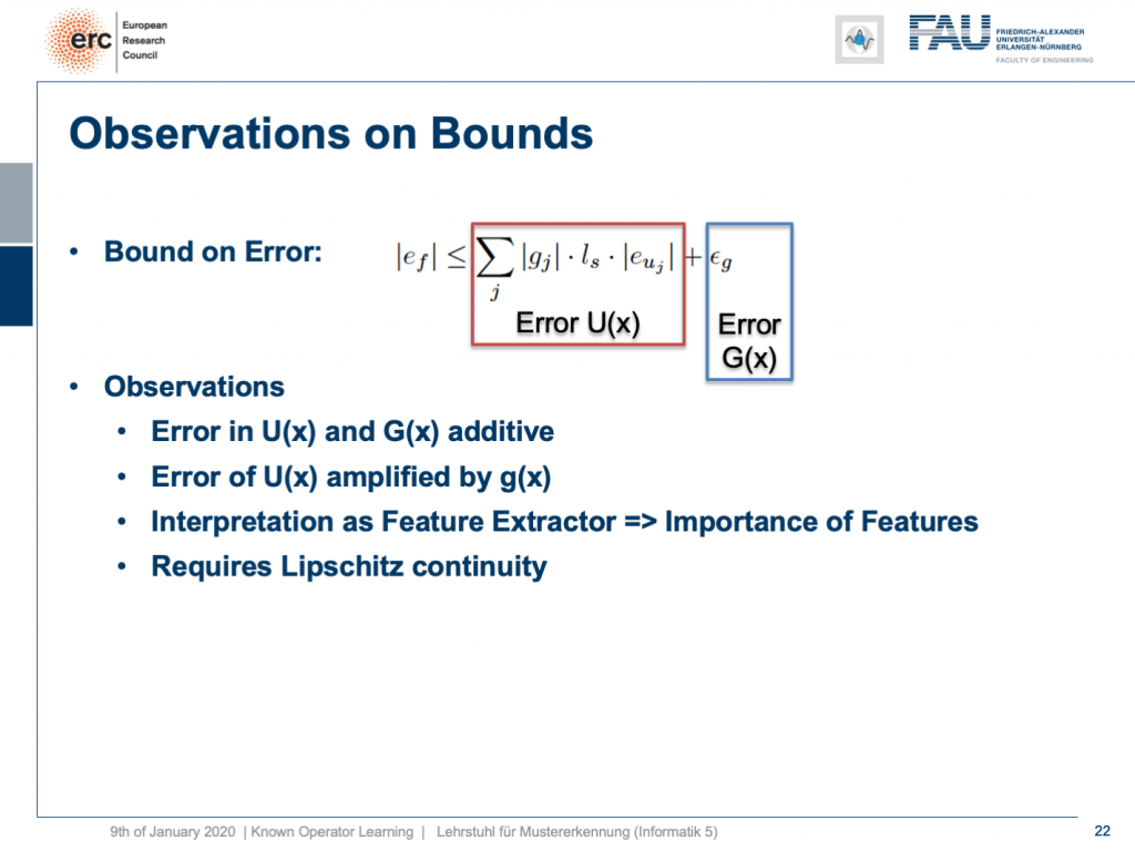
So, we can see that this bound has these very nice properties. If we now relate this to classical pattern recognition, then we could interpret u(x) as a feature extractor and g(x) as a classifier. So, you see that if we do errors in u(x), they get potentially amplified by g(x). This also gives us hints why in classical pattern recognition there was this very high focus on feature extraction. Any feature that you don’t extract correctly, is simply missing. This is also a big advantage of our deep learning approaches. We can also optimize the feature extraction with respect to the classification. Note that when deriving all of this we required Lipschitz continuity.

Okay. Now, you may say “This is only for two layers!”. We also extended this for deep networks. So, you can actually do this. Once you have the two-layer constellation, you can find a proof by recursion that there’s also a bound for deep networks. Then, you essentially get a sum over the layers to find this upper bound. It still holds that it’s the error that is introduced by the respective layer that contributes in an additive way to the total error bound. Again, if I know one layer that part of the error is gone, and the total upper bound is reduced nicely. We managed to publish this in nature machine intelligence. So, seemingly this was an interesting result also for other researchers. Okay. Now, we talked about the theory of why it makes sense to include known operations into deep networks. So, it’s not just common sense knowledge that we want to reuse these priors, but we can actually formally show that we’re reducing the error bounds.

So in the next lecture, we want to look into a couple of examples of this. Then, you will also see how many different applications actually use this. So, thank you very much for listening and see you in the next video. Bye-bye!

If you liked this post, you can find more essays here, more educational material on Machine Learning here, or have a look at our Deep LearningLecture. I would also appreciate a follow on YouTube, Twitter, Facebook, or LinkedIn in case you want to be informed about more essays, videos, and research in the future. This article is released under the Creative Commons 4.0 Attribution License and can be reprinted and modified if referenced. If you are interested in generating transcripts from video lectures try AutoBlog.

Thanks

Many thanks to Weilin Fu, Florin Ghesu, Yixing Huang Christopher Syben, Marc Aubreville, and Tobias Würfl for their support in creating these slides.

References

[1] Florin Ghesu et al. Robust Multi-Scale Anatomical Landmark Detection in Incomplete 3D-CT Data. Medical Image Computing and Computer-Assisted Intervention MICCAI 2017 (MICCAI), Quebec, Canada, pp. 194-202, 2017 – MICCAI Young Researcher Award
[2] Florin Ghesu et al. Multi-Scale Deep Reinforcement Learning for Real-Time 3D-Landmark Detection in CT Scans. IEEE Transactions on Pattern Analysis and Machine Intelligence. ePub ahead of print. 2018
[3] Bastian Bier et al. X-ray-transform Invariant Anatomical Landmark Detection for Pelvic Trauma Surgery. MICCAI 2018 – MICCAI Young Researcher Award
[4] Yixing Huang et al. Some Investigations on Robustness of Deep Learning in Limited Angle Tomography. MICCAI 2018.
[5] Andreas Maier et al. Precision Learning: Towards use of known operators in neural networks. ICPR 2018.
[6] Tobias Würfl, Florin Ghesu, Vincent Christlein, Andreas Maier. Deep Learning Computed Tomography. MICCAI 2016.
[7] Hammernik, Kerstin, et al. “A deep learning architecture for limited-angle computed tomography reconstruction.” Bildverarbeitung für die Medizin 2017. Springer Vieweg, Berlin, Heidelberg, 2017. 92-97.
[8] Aubreville, Marc, et al. “Deep Denoising for Hearing Aid Applications.” 2018 16th International Workshop on Acoustic Signal Enhancement (IWAENC). IEEE, 2018.
[9] Christopher Syben, Bernhard Stimpel, Jonathan Lommen, Tobias Würfl, Arnd Dörfler, Andreas Maier. Deriving Neural Network Architectures using Precision Learning: Parallel-to-fan beam Conversion. GCPR 2018. https://arxiv.org/abs/1807.03057
[10] Fu, Weilin, et al. “Frangi-net.” Bildverarbeitung für die Medizin 2018. Springer Vieweg, Berlin, Heidelberg, 2018. 341-346.
[11] Fu, Weilin, Lennart Husvogt, and Stefan Ploner James G. Maier. “Lesson Learnt: Modularization of Deep Networks Allow Cross-Modality Reuse.” arXiv preprint arXiv:1911.02080 (2019).

Category: Lecture Notes in Deep Learning