
Don’t re-invent the Wheel
These are the lecture notes for FAU’s YouTube Lecture “Deep Learning“. This is a full transcript of the lecture video & matching slides. We hope, you enjoy this as much as the videos. Of course, this transcript was created with deep learning techniques largely automatically and only minor manual modifications were performed. Try it yourself! If you spot mistakes, please let us know!
Welcome back to deep learning, So today, I want to talk to you about ideas on how we can reuse prior knowledge and integrate it into deep networks. This is actually something that we’ve been doing in a large research project that is being funded by the European Research Council and I thought these ideas are also interesting for you.
So, I decided to include them in the lecture. This brings us to the topic of known operator learning. Known operator learning is a very different approach because we try to reuse knowledge that we already have about the problem. Therefore, we have to learn fewer parameters. This is very much in contrast to what we know from traditional deep learning. If you say so traditional deep learning, then we often try to learn everything from the data. Now, the reason why we want to learn everything from the data is, of course, because we know very little about how the network is actually supposed to look like. So, we try to learn everything from the data in order to get rid of bias. In particular, this is the case for perceptual tasks where we have very little knowledge of how humans actually solve the problem. The human brain for us is largely a black box and we try to find a matching black box that is also solving the problem.
I brought this example here from Florin Ghesu, and you remember, I showed this already in the introduction. Here, we had this kind of reinforcement learning-type approach where we then motivate our search for organs in the body by reinforcement learning. We look at small patches in the image and then decide where to move in the next step in order to approach the specific landmark. So, we kind of can introduce here how we interpret the image or how a radiologist interprets the image and how he would move towards a certain landmark. Of course, we had this multi-scale approach. The main reason, why we do it in this way is, of course, because we don’t know how the brain actually works and what the radiologist is actually thinking. But we can at least mimic his working style in the way how we approach this here. Well, but this is generally not the case for all problems. Deep learning is so popular that it’s being applied to many, many, different problems other than perceptual tasks.
For example, people have been using this in order to model CT reconstruction. So here, the problem is that you have a set of projection data shown here on the left and you want to reconstruct slice data shown on the right-hand side.
The problem is very well researched on. We know solutions to this problem already since 1917 but there are, of course, problems of artifacts and image quality, and so on, dynamics which make the problem hard. Therefore, we would like to find improved reconstruction methods.
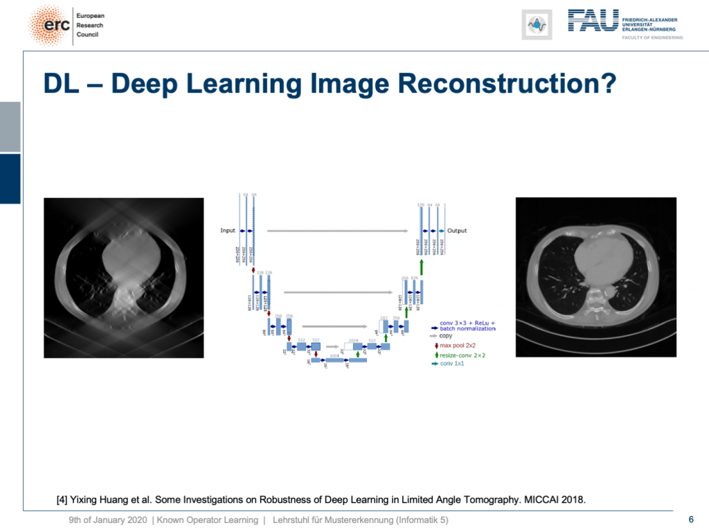
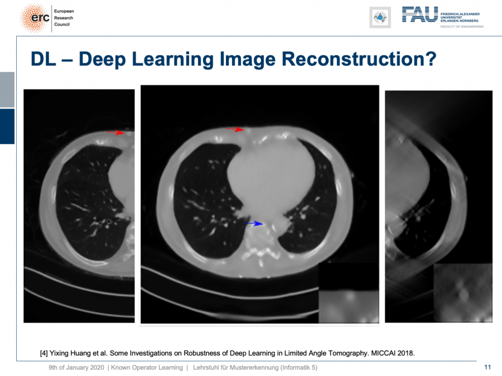
One problem, for example, is called the limited angle problem. If we only rotate by let’s say 120 degrees instead of a full rotation, you get slice images like shown here on the left-hand side. They are full of artifact and you can barely see what is shown on the image. We have the matching slice image on the right-hand side. If you look at the right-hand side image, you can see this is a cut through the torso. It shows the lungs, it shows the heart, it shows the spine, and ribs in the front. We barely see the ribs and the spine in the image on the left, but we have methods that can do image to image completion. We’ve seen that we can even use this for inpainting to interpolate missing information in images. So why not just apply it to complete the reconstruction? This has actually been done.
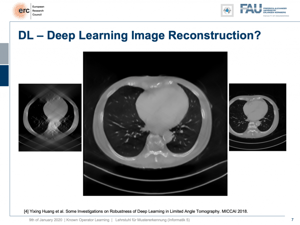
I can show you one result here. So, this actually works. This is done for an unseen person. So, this has been trained with slices from 10 other persons and evaluated here on the 11th one. So, this person has never been seen and you can see it very nicely reconstructs the ribs, the torso, the chest wall is there that is barely visible in the input image. We can also see a very nice appearance here. So, this is pretty cool. But to be honest: This is a medical image. People do diagnosis on this.
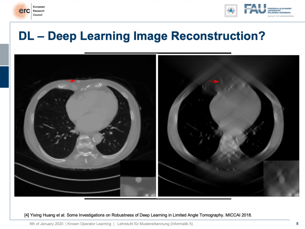
So, let’s put it a bit to the test and hide a lesion. So, we put it here exactly in the chest wall and this is kind of mean because this is exactly where we had the worst image quality. I’m also showing a blow-up view on the bottom right, so you see that the lesion is there and it has considerably higher contrast than the surrounding tissue. Now, if I show you this, you can see the input that we would show to our U-net on the right. So, you can see the lesion is barely visible in the blow-up view. You can actually see it, but it has a lot of artifacts. Now, the question is will it be preserved or will it be removed from the image?
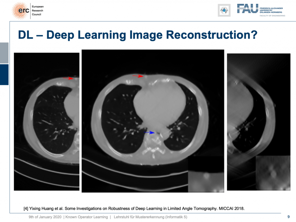
Well, it’s there! You can see the lesion is here. So that’s pretty cool, but what you can also see is the blue arrow. There hasn’t been a hole previously. So somehow this is also a bit unsettling. So, we actually looked into more details and into the robustness as you can see here in [4].

We did adversarial attacks on these kinds of networks. The most surprising adversarial attack is actually if you provide Poisson noise, the noise that realistically would appear in the projection data. Then, you get this. If I switch now a bit back and forth, you can see how the chest wall moves by approximately 1 centimeter. It still is an appealing image, but the lesion is entirely gone and the only thing we did is we added a bit of noise to the input data. Well, of course, the reason why it breaks this much is because we never trained with noise and the network has never seen these noise patterns. This is why it broke.
So, if we add Poisson noise to the input data, then you can also see we get a much better result. The chest wall is where but it’s supposed to be, but our lesion isn’t as clear as it used to be. To be honest, if you do medical diagnosis on this, it will be very hard because you don’t have the faintest idea where artifacts are because the artifacts don’t look artificial anymore. So you can’t recognize them that well.
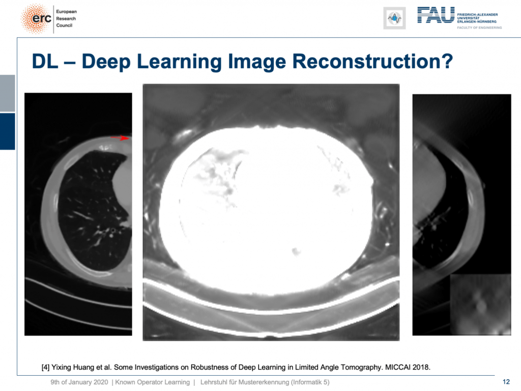
By the way, you remember that we have to deal with local minima in our optimization process. In one of the training runs, we got a network that would produce images like this one. So, we now window-leveled into the background of the patient. You can see that this kind of network started painting organ-like shapes like livers and kidneys into the air beside the patient. So, you may want to think about whether this is such a great idea to do complete black box learning on image reconstruction.
This is why we will talk next time about some ideas to incorporate prior knowledge into our deep networks. So, I hope you liked this video and I am hoping to see you in the next one. Bye-bye!
If you liked this post, you can find more essays here, more educational material on Machine Learning here, or have a look at our Deep LearningLecture. I would also appreciate a follow on YouTube, Twitter, Facebook, or LinkedIn in case you want to be informed about more essays, videos, and research in the future. This article is released under the Creative Commons 4.0 Attribution License and can be reprinted and modified if referenced. If you are interested in generating transcripts from video lectures try AutoBlog.
Thanks
Many thanks to Weilin Fu, Florin Ghesu, Yixing Huang Christopher Syben, Marc Aubreville, and Tobias Würfl for their support in creating these slides.
References
[1] Florin Ghesu et al. Robust Multi-Scale Anatomical Landmark Detection in Incomplete 3D-CT Data. Medical Image Computing and Computer-Assisted Intervention MICCAI 2017 (MICCAI), Quebec, Canada, pp. 194-202, 2017 – MICCAI Young Researcher Award
[2] Florin Ghesu et al. Multi-Scale Deep Reinforcement Learning for Real-Time 3D-Landmark Detection in CT Scans. IEEE Transactions on Pattern Analysis and Machine Intelligence. ePub ahead of print. 2018
[3] Bastian Bier et al. X-ray-transform Invariant Anatomical Landmark Detection for Pelvic Trauma Surgery. MICCAI 2018 – MICCAI Young Researcher Award
[4] Yixing Huang et al. Some Investigations on Robustness of Deep Learning in Limited Angle Tomography. MICCAI 2018.
[5] Andreas Maier et al. Precision Learning: Towards use of known operators in neural networks. ICPR 2018.
[6] Tobias Würfl, Florin Ghesu, Vincent Christlein, Andreas Maier. Deep Learning Computed Tomography. MICCAI 2016.
[7] Hammernik, Kerstin, et al. “A deep learning architecture for limited-angle computed tomography reconstruction.” Bildverarbeitung für die Medizin 2017. Springer Vieweg, Berlin, Heidelberg, 2017. 92-97.
[8] Aubreville, Marc, et al. “Deep Denoising for Hearing Aid Applications.” 2018 16th International Workshop on Acoustic Signal Enhancement (IWAENC). IEEE, 2018.
[9] Christopher Syben, Bernhard Stimpel, Jonathan Lommen, Tobias Würfl, Arnd Dörfler, Andreas Maier. Deriving Neural Network Architectures using Precision Learning: Parallel-to-fan beam Conversion. GCPR 2018. https://arxiv.org/abs/1807.03057
[10] Fu, Weilin, et al. “Frangi-net.” Bildverarbeitung für die Medizin 2018. Springer Vieweg, Berlin, Heidelberg, 2018. 341-346.
[11] Fu, Weilin, Lennart Husvogt, and Stefan Ploner James G. Maier. “Lesson Learnt: Modularization of Deep Networks Allow Cross-Modality Reuse.” arXiv preprint arXiv:1911.02080 (2019).