CT Reconstruction Revisited
These are the lecture notes for FAU’s YouTube Lecture “Deep Learning“. This is a full transcript of the lecture video & matching slides. We hope, you enjoy this as much as the videos. Of course, this transcript was created with deep learning techniques largely automatically and only minor manual modifications were performed. Try it yourself! If you spot mistakes, please let us know!
Welcome back to deep learning! So today, we want to look into the applications of known operator learning and a particular one that I want to show today is CT reconstruction.
So here, you see the formal solution to the CT reconstruction problem. This is the so-called filtered back-projection or Radon inverse. This is exactly the equation that I referred to earlier that has already been solved in 1917. But as you may know, CT scanners have only been realized in 1971. So actually, Radon who found this very nice solution has never seen it put to practice. So, how did he solve the CT reconstruction problem? Well, CT reconstruction is a projection process. It’s essentially a linear system of equations that can be solved. The solution is essentially described by a convolution and a sum. So, it’s a convolution along the detector direction s and then a back-projection over the rotation angle θ. During the whole process, we suppress negative values. So, we kind of also get a non-linearity into the system. This all can also be expressed in matrix notation. So, we know that the projection operations can simply be described as a matrix A that describes how the rays intersect with the volume. With this matrix, you can simply take the volume x multiplied with A and this gives you the projections p that you observe in the scanner. Now, getting the reconstruction is you take the projections p and you essentially need some kind of inverse or pseudo-inverse of A in order to compute this. We can see that there is a solution that is very similar to what we’ve seen in the above continuous equation. So, we have essentially a pseudo-inverse here and that is A transpose times A A transpose inverted times p. Now, you could argue that the inverse that you see here in a is actually the filter. So, for this particular problem, we know that the inverse of A A transpose will form a convolution.
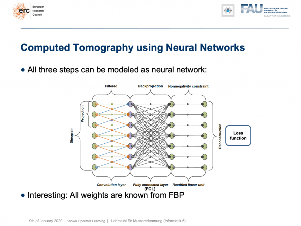
This is nice because we know how to implement convolutions into deep networks, right? Matrix multiplications! So, this is what we did. We can map everything into a neural network. We start on the left-hand side. We put in the Sinogram, i.e., all of the projections. We have a convolutional layer that is computing the filtered projections. Then, we have a back-projection that is a fully connected layer and it’s essentially this large matrix A. Finally, we have the non-negativity constraint. So essentially, we can define a neural network that does exactly filtered back-projection. Now, this is actually not so super interesting because there’s nothing to learn. We know all of those weights and by the way, the matrix A is really huge. For 3-D problems, it can approach up to 65,000 terabytes of memory in floating-point precision. So, you don’t want to instantiate this matrix. The reason why you don’t want to do that it that it’s very sparse. So, only a very small fraction of the elements in A are actual connections. This is very nice for CT reconstruction because then you typically never instantiate A but you compute A and A transpose simply using raytracers. This is typically done on a graphics board. Now, why are we talking about all of this? Well, we’ve seen there are cases where CT reconstruction is insufficient and we could essentially do trainable CT reconstruction.
Already, if you look at a CT book, you run into the first problems. If you implement it by the book and you just want to reconstruct a cylinder that is merely showing the value of one within this round area, then you would like to have an image like this one where everything is one within the cylinder and outside of the cylinder it’s zero. So, we’re showing this line plot here along the blue line through the original slice image. Now, if you just implement filtered back-projection, as you find it in the textbook, you get a reconstruction like this one. The typical mistake is that you choose the length of the Fourier transform too short and the other one is that you don’t consider the discretization appropriately. Now, you can work with this and fix the problem in the discretization. So what you can do now is essentially train the correct filter using learning techniques. So, what you would do in a classical CT class is you would run through all the math from the continuous integration to the discrete version in order to figure out the correct filter coefficients.
Instead, here we show that by knowing that it takes the form of convolution, we can express our inverse simply as p times the Fourier transform which is also just a matrix multiplication F. Then, K is a diagonal matrix that holds the spectral weights followed an inverse Fourier transform that is denoted as F hermitian here. Lastly, you back-project. We can simply write this up as a set of matrices and by the way, this would then also define the network architecture. Now, we can actually optimize the correct filter weights. What we have to do is we have to solve the associate optimization problem. This is simply to have the right-hand side equal to the left-hand side and we choose an L2 loss.
You’ve seen that on numerous occasions in this class. Now, if we do that, we can also compute this by hand. If you use the matrix cookbook then, you get the following gradient with respect to the layer K. This would be F times A times and then in brackets A transpose F hermitian our diagonal filter matrix K times the Fourier transform times p minus x and then times F times p transpose. So if you look at this, you can see that this is actually the reconstruction. This is the forward pass through our network. This is the error that is introduced. So, this is our sensitivity that we get at the end of the network if we apply our loss. We compute the sensitivity and then we backpropagate up to the layer where we actually need it. This is layer K. Then, we multiply with the activations that we have in this particular layer. If you remember our lecture on feed-forward networks, this is nothing else than the respective layer gradient. We still can reuse the math that we learned in this lecture very much earlier. So actually, we don’t have to go through the pain of computing this gradient. Our deep learning framework will do it for us. So, we can save a lot of time using the backpropagation algorithm.
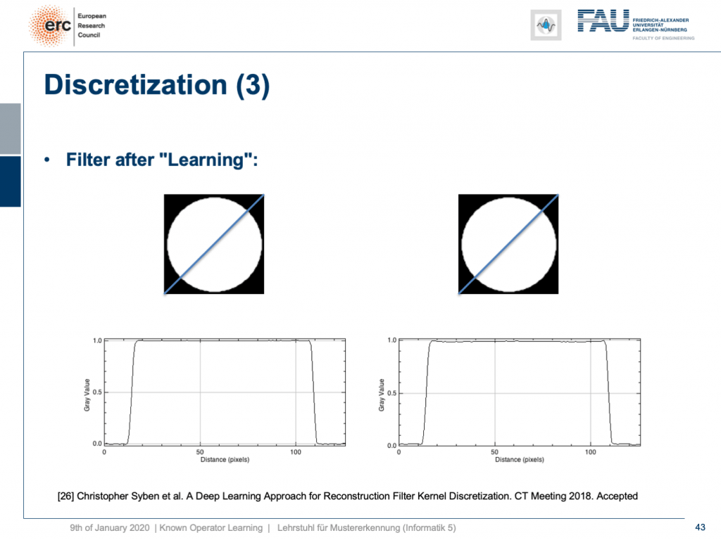
What happens if you do so? Well, of course, after learning the artifact is gone. So, you can remove this artifact. Well, this is kind of an academic example. We also have some more.
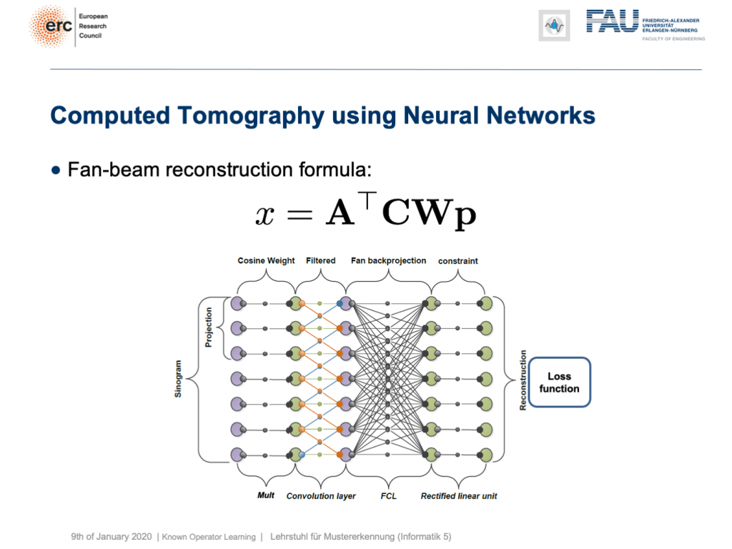
You can see that you can approximate also fan-beam reconstruction with similar matrix kinds of equations. We have now an additional matrix W. So, W is a point-wise weight that is multiplied to each pixel in the input image. C is now directly our convolutional matrix. So, we can describe a fan-beam reconstruction formula simply with this equation and of course, we can produce a resulting network out of this.
Now let’s look at what happens if we go back to this limited angle tomography problem. So, if you have a complete scan, it looks like this. Let’s go to a scan that has only 180 degrees of rotation. Here, the minimal set for the scan would be actually 200 degrees. So, we are missing 20 degrees of rotation. Not as strong as the limited angle problem that I showed in the introduction of known operator learning, but still significant artifact emerges here. Now, let’s take as pre-training our traditional filtered back-projection algorithm and adjust the weights and the convolution. If you do so, you get this reconstruction. So, you can see that the image quality is dramatically improved. A lot of the artifact is gone. There are still some artifacts on the right-hand side, but image quality is dramatically better. Now, you could argue “Well, you are again using a black box!”.
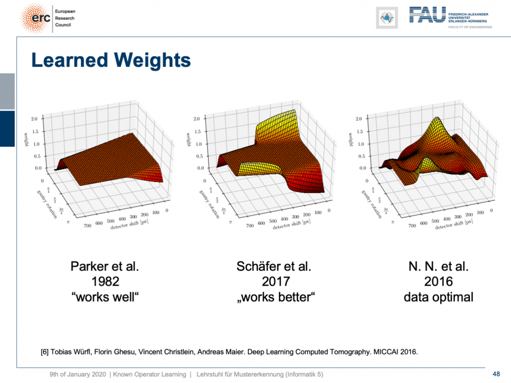
but that’s not actually true because our weights can be mapped back into the original interpretation. We still have a filtered back-projection algorithm. This means we can read out the trained weights from our network and compare them to the state-of-the-art. If you look here, we initialized with the so-called Parker weights which are the solution to a short scan. The idea here is that opposing rays are assigned a weight such that the rays that measure exactly the same line integrals essentially sum up to one. This is shown on the left-hand side. On the right-hand side, you find the solution that our neural network found in 2016. So this is the data-optimal solution. You see it did significant changes to our Parker weights. Now, in 2017 Schäfer et al. published a heuristic how to fix these limited angle artifacts. They suggested ramping up the weight of rays that run through the area where we are missing observations. They simply increase the weight in order to fix the deterministic mass loss. What they found looks better, but is a heuristic. We can see that our neural network found a very similar solution and we can demonstrate that this is data-optimal. So, you can see a distinct difference on the very left and the very light right. If you look here and if you look here, you can see that in these weights, this goes all the way up here and here. This is actually the end of the detector. So, here and here is the boundary of the detector, also here and here. This means we didn’t have any change in these areas here and these areas here. The reason for that is we never had an object in the training data that would fill the entire detector. Hence, we can also not backpropagate gradients here. This is why we essentially have the original initialization still at these positions. That’s pretty cool. That’s really interpreting networks. That’s really understanding what’s happening in the training process, right?
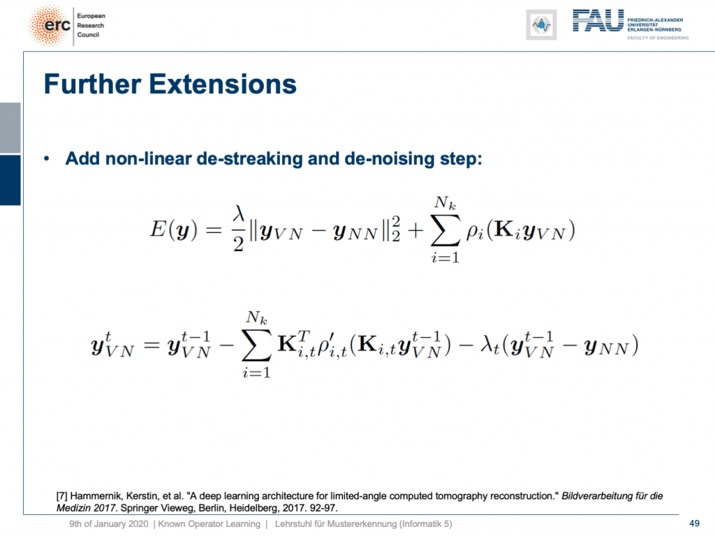
So, can we do more? Yes, there are even other things like so-called variational networks. This is work by Kobler, Pock, and Hammernik and they essentially showed that any kind of energy minimization can be mapped into a kind of unrolled, feed-forward problem. So, essentially an energy minimization can be solved by gradient descent. So, you essentially end up with an optimization problem that you seek to minimize. If you want to do that efficiently, you could essentially formulate this as a recurrent neural network. How did we deal with recurrent neural networks? Well, we unroll them. So any kind of energy minimization can be mapped into a feed-forward neural network, if you fix the number of iterations. This way, you can then take an energy minimization like this iterative reconstruction formula here or iterative denoising formula here and compute its gradient. If you do so, you will essentially end up with the previous image configuration minus the negative gradient direction. You do that and repeat this step by step.
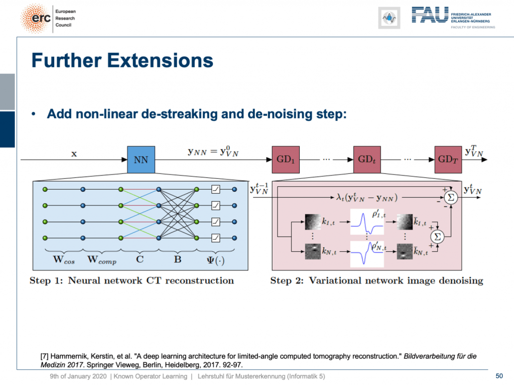
Here, we have a special solution because we combine it with our neural network reconstruction. We just want to learn an image enhancement step subsequently. So what we do is we take our neural network reconstruction and then hook up on the previous layers. There are T streaking or denoising steps that are trainable. They use compressed sensing theory. So, if you want to look into more details here, I recommend taking one of our image reconstruction classes. If you look into them you can see that there is this idea of compressing the image in a sparse domain. Here, we show that we can actually learn the transform that expresses the image contents in a sparse domain meaning that we can also get this new sparsifying transform and interpret it in a traditional signal processing sense.
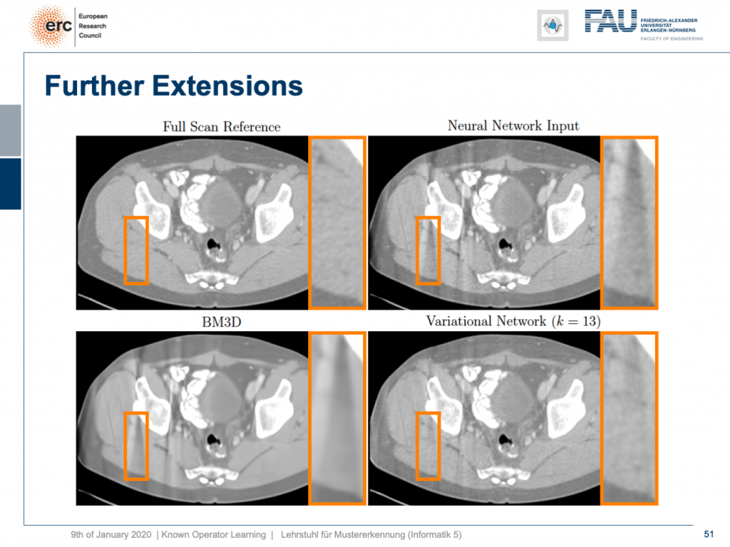
Let’s look at some results. Here, you can see that if we take the full scan reference, we get really an artifact-free image. Our neural network output with this reconstruction network that I showed earlier kind of is improved, but it still has these streak artifacts that you see on the top right. On the bottom left, you see the output of a denoising algorithm that is 3-D. So, this does denoising, but it still has problems with streaks. You can see that in our variational Network on the bottom right, the streaks are quite a bit suppressed. So, we really learn a transform based on the ideas of compressed sensing in order to remove those streaks. A very nice neural network that mathematically exactly models a compressed sensing reconstruction approach. So that’s exciting!
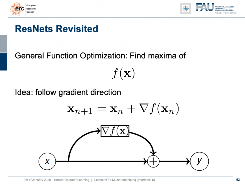
By the way, if you think of this energy minimization idea, then you also find the following interpretation: The energy minimization and this unrolling always lead to a ResNet because you take the previous configuration minus the negative gradient direction meaning that it’s the previous layers output plus the new layer’s configuration. So, this essentially means that ResNets can also be expressed in this kind of way. They always are the result of any kind of energy minimization problem. It could also be a maximization. In any case, we don’t even have to know whether it’s a maximization or minimization, but generally, if you have a function optimization, then you can always find the solution to this optimization process through a ResNet. So, you could argue that ResNets are also suited to find the optimization strategy for a completely unknown error function.
Interesting, isn’t it? Well, there are a couple of more things that I want to tell you about these ideas of known operator learning. Also, we want to see more applications where we can apply this and maybe also some ideas on how the field of deep learning and machine learning will evolve over the next couple of months and years. So, thank you very much for listening and see you in the next and final video. Bye-bye!
If you liked this post, you can find more essays here, more educational material on Machine Learning here, or have a look at our Deep LearningLecture. I would also appreciate a follow on YouTube, Twitter, Facebook, or LinkedIn in case you want to be informed about more essays, videos, and research in the future. This article is released under the Creative Commons 4.0 Attribution License and can be reprinted and modified if referenced. If you are interested in generating transcripts from video lectures try AutoBlog.
Thanks
Many thanks to Weilin Fu, Florin Ghesu, Yixing Huang Christopher Syben, Marc Aubreville, and Tobias Würfl for their support in creating these slides.
References
[1] Florin Ghesu et al. Robust Multi-Scale Anatomical Landmark Detection in Incomplete 3D-CT Data. Medical Image Computing and Computer-Assisted Intervention MICCAI 2017 (MICCAI), Quebec, Canada, pp. 194-202, 2017 – MICCAI Young Researcher Award
[2] Florin Ghesu et al. Multi-Scale Deep Reinforcement Learning for Real-Time 3D-Landmark Detection in CT Scans. IEEE Transactions on Pattern Analysis and Machine Intelligence. ePub ahead of print. 2018
[3] Bastian Bier et al. X-ray-transform Invariant Anatomical Landmark Detection for Pelvic Trauma Surgery. MICCAI 2018 – MICCAI Young Researcher Award
[4] Yixing Huang et al. Some Investigations on Robustness of Deep Learning in Limited Angle Tomography. MICCAI 2018.
[5] Andreas Maier et al. Precision Learning: Towards use of known operators in neural networks. ICPR 2018.
[6] Tobias Würfl, Florin Ghesu, Vincent Christlein, Andreas Maier. Deep Learning Computed Tomography. MICCAI 2016.
[7] Hammernik, Kerstin, et al. “A deep learning architecture for limited-angle computed tomography reconstruction.” Bildverarbeitung für die Medizin 2017. Springer Vieweg, Berlin, Heidelberg, 2017. 92-97.
[8] Aubreville, Marc, et al. “Deep Denoising for Hearing Aid Applications.” 2018 16th International Workshop on Acoustic Signal Enhancement (IWAENC). IEEE, 2018.
[9] Christopher Syben, Bernhard Stimpel, Jonathan Lommen, Tobias Würfl, Arnd Dörfler, Andreas Maier. Deriving Neural Network Architectures using Precision Learning: Parallel-to-fan beam Conversion. GCPR 2018. https://arxiv.org/abs/1807.03057
[10] Fu, Weilin, et al. “Frangi-net.” Bildverarbeitung für die Medizin 2018. Springer Vieweg, Berlin, Heidelberg, 2018. 341-346.
[11] Fu, Weilin, Lennart Husvogt, and Stefan Ploner James G. Maier. “Lesson Learnt: Modularization of Deep Networks Allow Cross-Modality Reuse.” arXiv preprint arXiv:1911.02080 (2019).