System Theory – Introduction to Fourier Series and Transform

These are the lecture notes for FAU’s YouTube Lecture “Medical Engineering“. This is a full transcript of the lecture video & matching slides. We hope, you enjoy this as much as the videos. Of course, this transcript was created with deep learning techniques largely automatically and only minor manual modifications were performed. Try it yourself! If you spot mistakes, please let us know!

Welcome back to Medical Engineering: Medical Imaging Systems. So today we want to talk about the key concept of systems theory and this is the so-called Fourier series and Fourier transform. You will see that this one will pop up in your entire study program. You will need Fourier Transforms really frequently all the time and it’s a very very nice tool to understand functions and calculating the functions. So it’s a really cool concept already 250 years old but still very very relevant for our field. So looking forward to exploring with you the  Fourier series and the Fourier transform.

Okay so let’s have a look at the Fourier series and the Fourier transform. Let’s start with the Fourier series. 

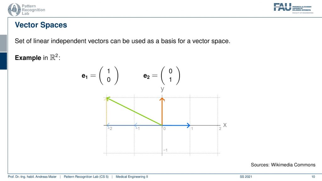
Now what we want to introduce is essentially something like an equivalent thing to a vector space and here we have the example of the vector space. So you see this little figure here if we want to describe some arrows in 2d then we can use a vector space in order to represent that error. That arrow is essentially mapped onto bases. So here our 2d vector basis is given by two vectors that are e1 and e2. If I know e1 and e2 I can express any other vector in that plane as a linear combination of the two. So I multiply e1 with some value and then multiply e2 with some value and add them and I get essentially one point in that 2d plane. So here if you look at the green arrow you see that I have to multiply the red arrow once and then add the blue arrow multiply it with -2 to it such that I get exactly the green arrow. So the idea of the Fourier series is now to expand this concept to function spaces. So this is a kind of abstract concept, isn’t it? 

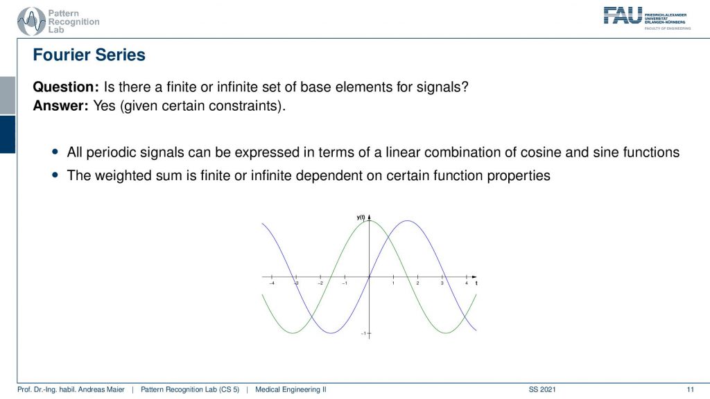
But let’s look into some examples. So we want to have some kind of basis for signals and now signals are functions that are some f(t). So it’s dependent on some time t and we want to be able to express this function somehow with a kind of basis. Now the question is if this is possible at all and the answer is yes given some certain constraints. The key idea now is that we want to express periodic signals and all periodic signals can be expressed in terms of linear combinations. So you multiply with a certain weight cosine and sine functions and add them up. So the weighted sum can be finite or infinite depending on the properties of the signal. But the combination of different sine waves of different frequencies or wavelengths is then able to approximate any kind of periodic signal. That is a pretty interesting observation, isn’t it? Do you believe that? Well, I’ll show it with a short example.

 So let’s look at this function here.

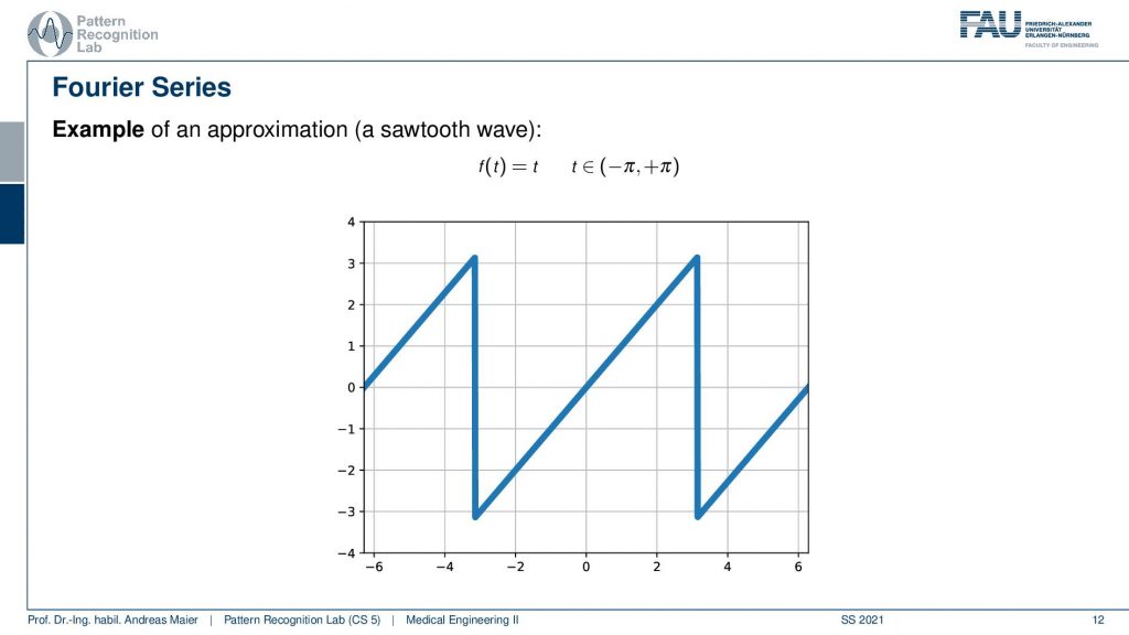
 This function here is a sawtooth and the sawtooth wave can be mathematically expressed as a linear increase within a certain period. Then it simply repeats. Now, this sawtooth wave can be expressed as sine functions. Let’s have a look at this. 

So this is now one sine wave and you see it kind of approximates our sawtooth but it’s not a great fit right. So maybe one sine is not enough. So let’s add another sign and if we add a second sine wave, you see that our approximation kind of gets better. But it’s still coarse. So let’s add another one and another one and another one and another one and another one and another one and now you see that I kind of get better. But I still have to add quite a few of those sine waves in order to get there. Now, this is the approximation with 20, 29, 70. So I need quite a few of those sine waves but now I have sine waves of different wavelengths. I multiply them with a certain factor and add them up to approximate the red signal here and the blue signal was the one that I wanted to approximate and now the fit is already pretty good. So let’s have a look at this in a little more detail. 

So this is what we’re doing. We have our sawtooth wave and we want to approximate it with different sine waves and what we’re actually doing is we start with a simple sine wave that is simply the sin(t). Then we essentially adjust the wavelength. So we take another sine wave that has now half of the wavelength so this is 2 times t and then we add 3 times t, and 4 times t, and 5 times t, and 6 times t. Of course, we have to determine the correct coefficient for this and you see here that we essentially have to divide by 3, by 2 and by 5 π and so on in order to find the right coefficients. So we have different scaled sine waves and they have a different wavelength and increasing the wavelength we have to compute new coefficients for the weighted sum. But if I have the right coefficients I can start approximating this. Of course, I can go on and go on and go on and add more of these sine waves with increasing frequency and with an even shorter wavelength. You see that the approximation gets better. Now, this is essentially what we did to approximate the sawtooth here. Now you see here on the right-hand side the waves and on the left-hand side the approximation. So summed everything up. 

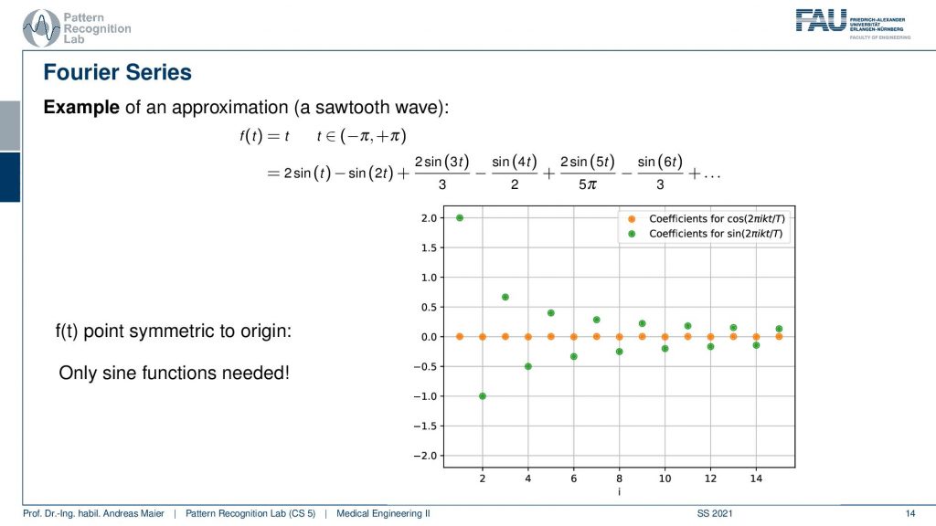
Let’s have a look also at the coefficients that I need to multiply the waves with. If I plot them here from 0 to increasing frequency or decreasing wavelength then you can see that I get the following pattern. So you see that I essentially get alternating points and these are the green ones for the sine waves, I get orange zeros everywhere for the cosine. So I’m only using sine waves here and I don’t need a single cosine in the weighted sum in order to do the approximation. Now, why is that? This is because f(t) is a point symmetric to the origin and this means that we only need sine functions for the approximation. Not a single cosine is needed here because our function that we desire to approximate, the sawtooth function is point symmetric to the origin.

Let’s have a look at one more example. 

Here we use a rectangular function over a certain period and here we have a different function. You see here that it is in the domain between zero and one. So we first start with one over two. So this is essentially the 0th frequency which is just the mean value. So we start with one over two. This is the red approximation. So this is essentially a sine wave without any frequency so this is just a flat graph. Then we start adding the cosines on top and you see if I add the first cosine then I actually need to determine a couple more coefficients and the next three coefficients all zero. Then I have another cosine that is added here and again three coefficients that are zero, another cosine that is added here, and then slowly my approximation gets better. You see in order to improve this approximation I have to add quite a few additional cosines in order to get a better approximation of our rectangular function here. 

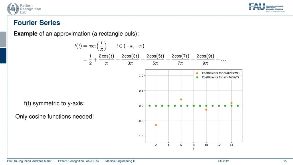
So let’s plot not just the cosines and the superposition of them, let’s also plot the coefficients over the frequency. Here you see that we have all of the sine coefficients now zero and only sometimes the cosine coefficients are nonzero values. You see that they are also alternating here and we need quite a few of them in order to approximate our function. So here f(t) is symmetric to the y axis and this means that only cosine functions are needed for the approximation. So that’s already an interesting observation and you’ll see that actually if you have something that is symmetric to the y-axis you will only need cosines and if you have something that is point symmetric to the origin then you only need sine functions in order to approximate those periodic functions. 

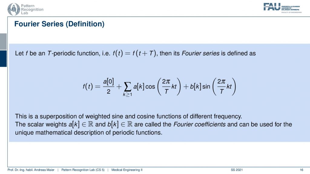
Now, what is this Fourier series? So the Fourier series is actually a kind of function approximation where we are using cosines and sines. Now we need a period duration of T and this is the duration of one period. Then we can find the Fourier series defined as the function that we wish to approximate f(t) is given as some coefficient a[0] over 2 plus a weighted sum of cosine and sine functions. Here a[k] is associated with the cosine and b[k] is associated with the sine. Now if you look into the bracket you see 2π over T times k times t. Now, 2π is essentially the length of your cosine or sine function and you divide it by the period length T in order to normalize for the respective period length. Now you have k times t, k is essentially giving the frequency of this wave and the higher you pick k the more lobes you will actually produce in the sine and cosine. Here t is simply the index of the function. So here we have a superposition of a weighted sum of sine and cosine functions of different frequencies and if I choose the a[k] and the b[k] correctly they will produce the original function. So now the key question is how can I determine the a[k] and the b[k]? These are called the Fourier coefficients. They are essentially unique mathematical descriptors of the periodic function.  

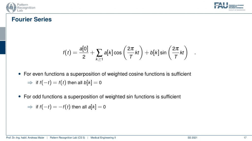
One more remark: for even functions the superposition of weighted cosine functions is sufficient. So here all the b[k]’s will be zero. In odd functions the superposition of weighted sine functions is sufficient and there all the a[k]’s will be zero. So this is what we’ve seen in the previous example. 

Now a key question is how we can actually compute those a[k] and b[k]? Now a[k] is determined as an integral from minus half the period length to plus half the period length and then you have essentially a pointwise multiplication of the function with the respective cosine wave of that particular frequency. The same is true for the b[k]. So for the b[k] of frequency k, you have to determine the integral from minus T over 2 to plus T over 2 and then you have a pointwise multiplication of the function with the respective sine wave. I have a little animation here for you. 

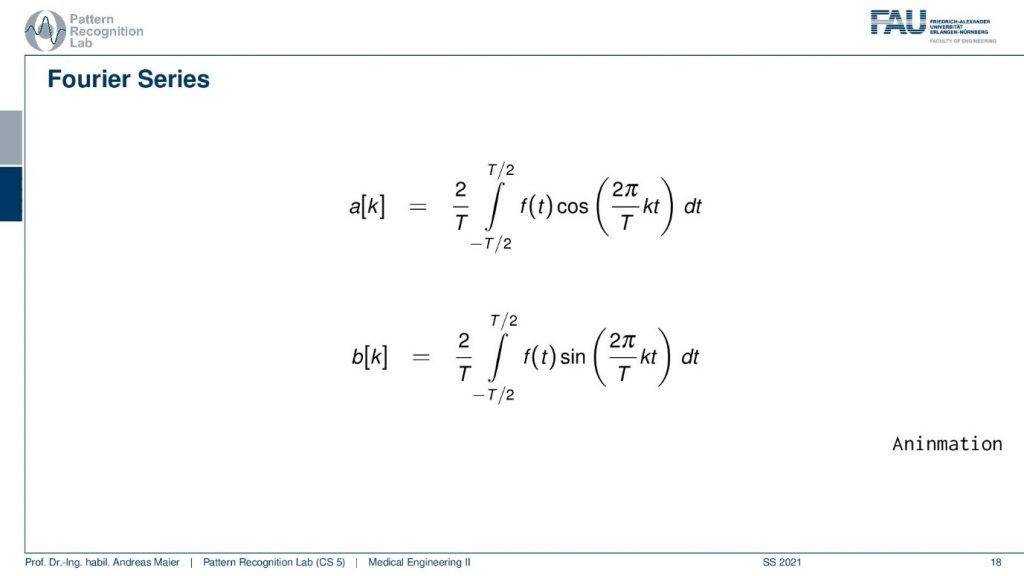
So here you can see a function and we are essentially determining the multiplication at every point. Then we add everything up that is what our integral is doing. Once we do that we get coefficients, we are plotting them here on the right-hand side. You can see that by multiplication step by step I get coefficients for different frequencies. The nice thing here is for these periodic functions you can visualize this in this way here. You see that by multiplication and sum of every frequency I get a coefficient. I actually can then reproduce the original function from only the frequency coefficients by multiplying them with the respective frequency and adding them up again. So this is a process that is invertible. So you could say that our sine and cosine functions are nothing else than a projection onto a specific basis. This basis is then able to represent a periodic function. That’s pretty cool, isn’t it? 

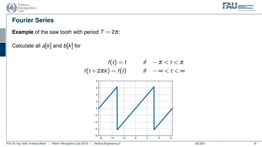
Let’s have a look at the Fourier series here. So here we did all the calculations and we showed the results. But actually, we would also like to determine our a[k] and b[k] for let’s say our sawtooth function. So how would we do that? Here we can then remember that this is an odd function. So all the a[k]’s will be zero. 

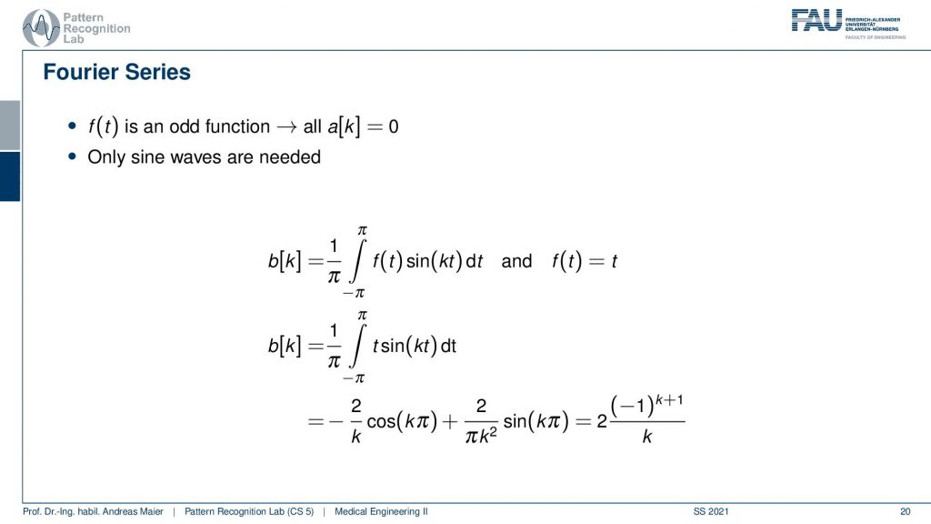
So we don’t have to deal with them. We only need to determine the sine wave coefficients. So these are our b[k]. Now we’ve seen that the b[k]’s can be computed as the respective period length. We know the period length here is 2π. So we have to plug this in for our integral. We integrate from -π to +π and this is the function times the sine function of the respective frequencies. Now let’s plug in our f(t) equals to t. Then we can see that we can compute the actual coefficients as the integral from -π to +π of t times our frequency. Fortunately, this has a closed-form solution that you find here at the bottom. This is how we can then determine our coefficients also analytically. So it’s not just that we have to determine this actually by having a computer evaluate this in a discrete way. This can also be determined completely analytically as in this example.

Now what we still have here are the sines and cosines that pop up and this notation is actually not used that much in literature. What people very often do is switch to Euler notation and you may remember that you can represent using complex numbers as a sum of cos(φ) plus isin(φ) as e to the power iφ.

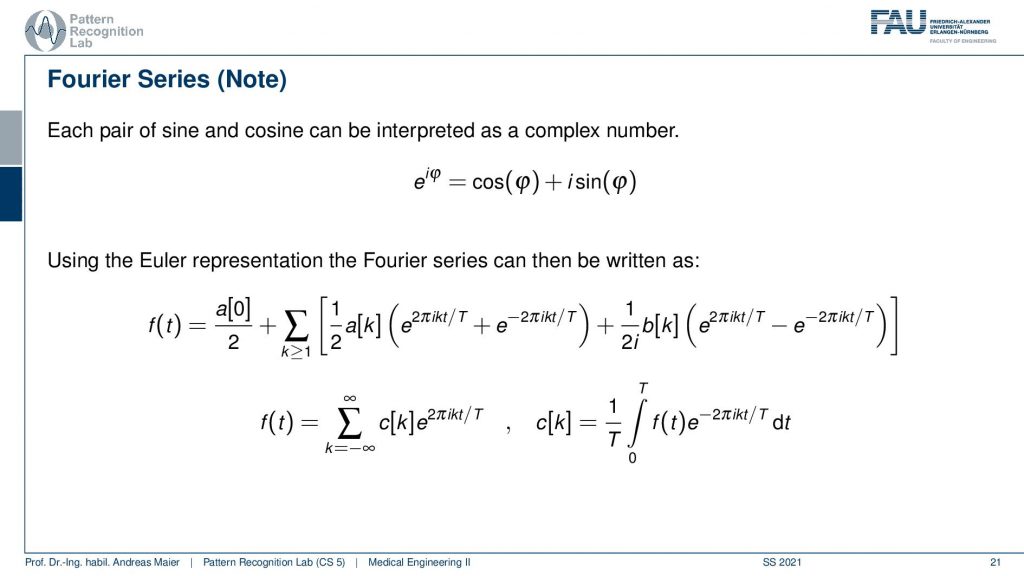
So this is the Euler representation of complex numbers and this is very very convenient because then we don’t have to deal with the a[k] and the b[k]. So we can plug this in with the definition of the cosine and the sine depending on the respective Euler representation. So this is what we did here in the center row and this actually allows us to find a representation that is then no longer using a[k] and b[k]. Instead, we are using a complex number that also has two coefficients. This is c[k] and you can see now that we represent the sum of the sine and cosine as the Euler function here. But this is an equivalent notation as we’ve seen earlier. But we don’t need the sine of the cosine but it’s just the e that is put in here. Of course, you then need the I in order to make sure that this is a complex number. Still, we can determine the c[k] as the integration from now 0 to T of the original function pointwise multiplied by the complex frequency here. So the projection onto the complex coefficients can still be done with this kind of projection. So it’s an integration and a multiplication. Okay so this is maybe a bit of math, but this way we can write things up in a very compact way. If you look into the coursebook that you find also in the video description, you will see that we actually also pieced out how to get from the a[k] and b[k] to the c[k]. In the coursebook there is a geek box. If you’re interested in math so I definitely recommend having a look at the book. 

This is already the summary of our Fourier series. So we can approximate functions using sine and cosine waves and we can then completely describe the function using the coefficients that are associated with the respective frequencies of sine and cosine waves. We have some special cases for odd and even functions. In the one, we only need sine, and the other one we only need cosine functions. The Fourier series might have finite or infinite terms. But all of this is only applicable to periodic functions. So Fourier series requires periodic functions. This theory already 250 years old still very very useful.

Now this periodicity constraint bothers us a little bit. 

So this is why we want to switch over to the Fourier transform and the Fourier transform addresses this question here. How can we extend the Fourier series to non-periodic signals? 

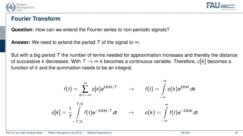
So the answer is well we extend the period simply from T to infinity and then it can be non-periodic because one-period length is just infinitely long. In an infinitely long period, you can represent every signal. So why not just do that? Well, one thing that is associated with a big period T is that the number of terms needed for the approximation increases. This means that the distance of successive k decreases. So you have now really a long period length and the longer I take the period length the smaller is the distance between the different k’s in terms of frequency. Now if I go with the period length to infinity then k becomes a continuous variable because the distance between the individual steps of k goes towards zero. So, k becomes continuous. Now c[k] becomes a function of k and the summation needs to be integral. So you’ve seen that if we had previously with the Fourier series a sum of a discrete c[k], then we now need to convert this into an integral. The c[k] which had a discrete index for every k is now converted into a function c(k) which is now a continuous variable. So that’s the major change. You see it looks very similar other than we switch from discrete to continuous. This allows us now to have infinitely small distances between the frequencies. So we can have this at an infinite fine resolution. If we do so now we are able to analyze also signals of arbitrary length t.

Now what we get then here is the Fourier transform. 

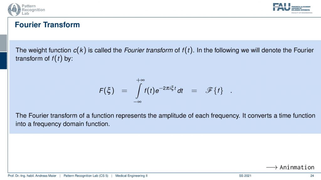
Now the Fourier transform is computing a weight function c(k) and this is the Fourier transform of f(t) and then the following we won’t use the c(k) anymore. But we will denote this by F(ξ) and now ξ is the continuous frequency variable and F is the Fourier transform. So now we get for continuous frequency variable values and they’re still computed as the integral but now from minus infinity to plus infinity because of the infinite period length of f(t) times and now our sine and cosine are wrapped up in this Euler notation and this is then e to the power of minus 2π. Here we need ξ for the frequency variable and t for the spatial domain variable. We integrate over dt and this delivers the Fourier transform of t. You see here that our Fourier transform is again a kind of system that we can apply. So the Fourier transform of a function represents the amplitude of each frequency. It converts a time function into a frequency domain function. So now we have two continuous variables- frequency variable ξ and the time variable t. If you are talking about images then the time variable is a spatial domain variable. So this is why people sometimes say this is a spatial domain and the Fourier domain. So this is often associated with images. If you’re talking about time-dependent functions then it’s the time domain. So sometimes people use that interchangeably. I also do.

So let’s have a look at an example.

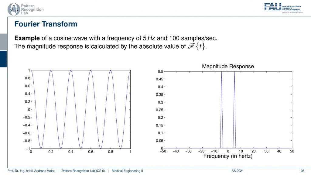
Let’s start off with a very simple example and we won’t go into too many mathematical details here. But let’s have a cosine wave with a frequency of 5 Hz at 100 samples per second and then the magnitude. So this is the cosine wave on the left-hand side and now we have the conversion into the Fourier domain so the magnitude response here on the right-hand side. You see that the Fourier transform is nothing else than exactly two peaks and these two peaks are located at exactly plus-minus 5 Hz. So this is the Fourier representation of the left signal. If I know Fourier’s representation then I can determine the other signal as well. So I can use them interchangeably. If I know the Fourier transform I can compute the original function and time domain and if I know the time domain I can compute the Fourier domain from that. So I can convert from one domain to another and this is essentially a base transform onto just a different set of base vectors. But now our base vectors are a continuous frequency variable. Why is this useful? Well, let’s look at a little more complex function.

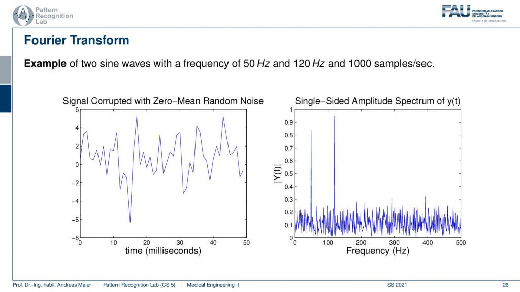
Here we actually have two sine waves and they have a frequency of 50Hz and 120Hz and a thousand samples per second. But we added this zero-mean random noise on top. Now if you look at the left-hand side if you see just a 50Hz wave and a 120 Hz wave, you would just want to see like two sine waves overlapping right? It doesn’t look like the left-hand side here. So this is kind of difficult to see the two sine waves here because of all of the noise. But now if I go to the frequency domain you can see that I can very clearly see the two peaks at 50 Hz and at 120 Hz. Note that I’m only showing the positive side. Now of the frequency space obviously there would also be a negative one, but I’m only showing the positive half-space here. But you can see the two peaks very distinctly and you also see that the zero-mean random noise loads into all of the frequencies and looking at this we actually have a very nice means now of getting rid of the noise right? So I could reconstruct the signal essentially perfectly if I put up a threshold on the frequency here and I just preserve the two peaks. Then I could reconstruct the original signal and this is exactly where the Fourier transform and also other things that we learn about in this class will be used for us. So we can recover the original signal by using tricks from signal processing. In particular, the Fourier transform is super useful for applications like denoising and so on. But it’s also a super useful tool to understand the systems. What they were actually doing and to work with the different systems of different properties. It’s a really really useful tool and just a hint that it will be useful for denoising. 

Okay so let’s summarize this a little bit. We have just seen that there is this concept of the Fourier series and the Fourier transform. I hope you could follow that both concepts stem from the idea that I want to find a basis, a kind of vector space like representation like we do in a 2d space where we have these base vectors and linear combinations of the base vectors are able to describe any point in that plane. We can also use sine and cosine functions to describe any periodic function as a weighted sum. Now if we want to get rid of the problem that they need to be periodic, we have to extend the period duration towards infinity. Then we get rid of the problem of being able to model only periodic functions. This comes essentially at the cost that we are no longer having sums of sines and cosines but our previous k is converted into a continuous variable that we then denoted as ξ. This is a continuous frequency variable that we can then use in order to describe this base vector representation. So it’s essentially a conversion into a different space and in this space, we can represent any kind of function as a superposition of sine and cosine waves. It’s a very very important concept and you will see that the Fourier transform regarding signals and systems will come up all the time. It’s a super useful tool that you should understand at some point maybe not after this video but you will see it comes up in your studies again and again. It’s very relevant for analyzing functions and describing signals and systems. In the next video, we will introduce another very important concept that is called convolution. This is also linked to systems theory and we will see that this is also linked to the Fourier transform in the next video. So I hope you enjoyed this little video and it brought to you some understanding of the Fourier transform and Fourier series and why we need those concepts. It was a bit math, I must admit that but I hope that the examples help you with understanding this concept of expressing functions by sine and cosine functions. So if you liked it please continue watching and we will see again in the next video where we talk about convolution. So thank you very much for watching and bye-bye!!

If you liked this post, you can find more essays here, more educational material on Machine Learning here, or have a look at our Deep Learning Lecture. I would also appreciate a follow on YouTube, Twitter, Facebook, or LinkedIn in case you want to be informed about more essays, videos, and research in the future. This article is released under the Creative Commons 4.0 Attribution License and can be reprinted and modified if referenced. If you are interested in generating transcripts from video lectures try AutoBlog

References  

1. P. Fischer, et al., “System Theory”, in Medical imaging systems: an introductory guide, edited by A. Maier, et al. (Springer International Publishing, Cham, 2018), pp. 13–36, 10.1007/978-3-319-96520-8_2  

Video References

1. 3Blue1Brown – What is a Fourier Transform? A Visual Introduction https://youtu.be/spUNpyF58BY
2. Continuous Fourier Transform of Rect and Sinc Functions https://commons.wikimedia.org/wiki/File:Continuous_Fourier_transform_of_rect_and_sinc_functions.gif

Kategorie: Lecture Notes in Medical Engineering