Lecture Notes in Pattern Recognition: Evaluation Measures and ROC Analysis

These are the lecture notes for FAU’s YouTube Lecture “Pattern Recognition“. This is a full transcript of the lecture video & matching slides. We hope, you enjoy this as much as the videos. Of course, this transcript was created with deep learning techniques largely automatically and only minor manual modifications were performed. Try it yourself! If you spot mistakes, please let us know!

Welcome everybody to a new round of pattern recognition questions and answers. Today we want to have a short chat about measures of evaluation classification systems and how a classification system can be altered in order to change the evaluation outcome. So I think you will find this interesting and I also brought a very interesting example to discuss the ideas of classification systems.

Today we want to discuss another round of questions and answers and in particular, we want to talk about the questions that you had sent them by email or posted in the forum. The key question that came up lately was can you discuss how do I evaluate a classification system?

So we talked about this in the lecture. But I found that we need some additional explanation to actually understand what the classification systems do and how we can evaluate them. So, of course, we will discuss this in an example. Everybody is talking about diseases nowadays and it seems everybody is becoming an expert on disease classification. So I also thought it would be interesting to talk about a typical disease and I took the zombie disease.

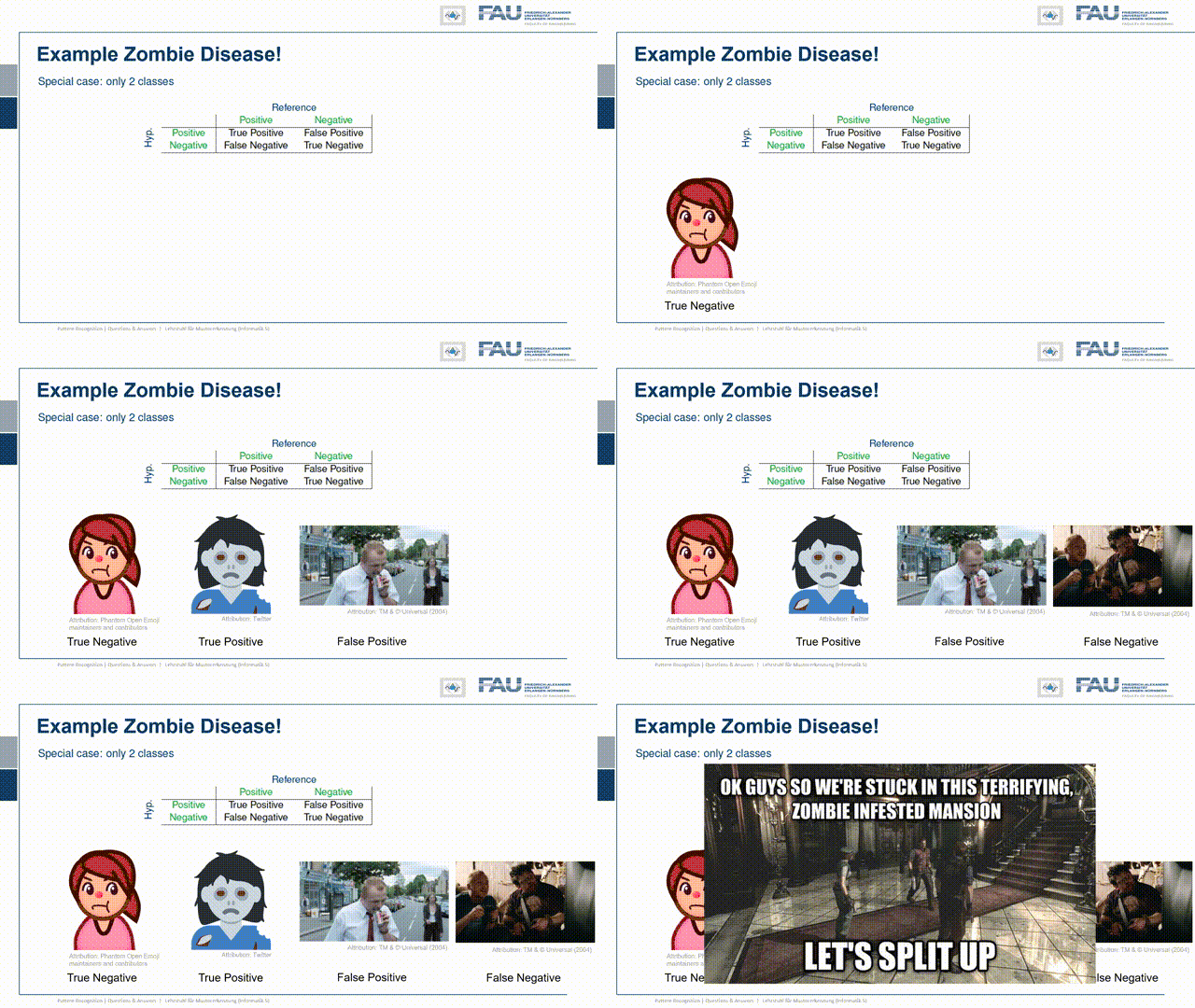
I think this is one of the most terrifying things that could happen to the world. So I think this is the right time to discuss what we should do when we encounter the zombie disease. You see here this is how we can evaluate then the outcome of a test. So we’re preparing already a test system to figure out who’s a zombie and who isn’t and we would of course then have a couple of possible outcomes and you know people could actually be zombies. So that would be the reference. So these are the columns or they could not be zombies. So they would be either positive or negative and then of course our classification result the hypothesis could then have one of the two outcomes. So this would then also be either positive or negative and of course, there are regular humans. So this is a true negative they are just regular humans and of course, the test results should also be negative for humans then of course we want our classification system to actually detect zombies. So there are factual zombies out there that we want to detect and we want the result to be also a zombie. So this would be a true positive. Now, of course, our classification system can also make mistakes, and then you know sometimes we detect somebody as a zombie who isn’t actually a zombie and I brought this small example here that you can memorize this. So this is from actually a very interesting horror movie “Shaun of the dead” and in the scene here, Shaun had a really bad hangover and he just goes out to the shop to buy a drink. You see he’s so severely hungover that he first of all he doesn’t realize or the walking dead around him and second they don’t recognize him because he behaves like one of them. So yeah this would be then a false positive. So people and luckily he also walking dead zombies think you are one of them and then there’s also the other case that we somehow miss that somebody is dead and has come back to life. Here is a situation where something like this is actually happening. So you know you’re involved in your favorite video game and you’re playing with your friend and at some point, you didn’t even realize that your friend has turned into a zombie and you’re still playing the video game. So this would be the case of a false negative. Now that we have understood what the different outcomes are and I hope you will be able to memorize this. So the false positive and the false negative are the two kinds of errors that we can do. So obviously I would never let you go unprepared into a terrible zombie disease. So, of course, I also have some advice for you. Okay guys we’re stuck in this terrifying zombie-infected mansion let’s split up.

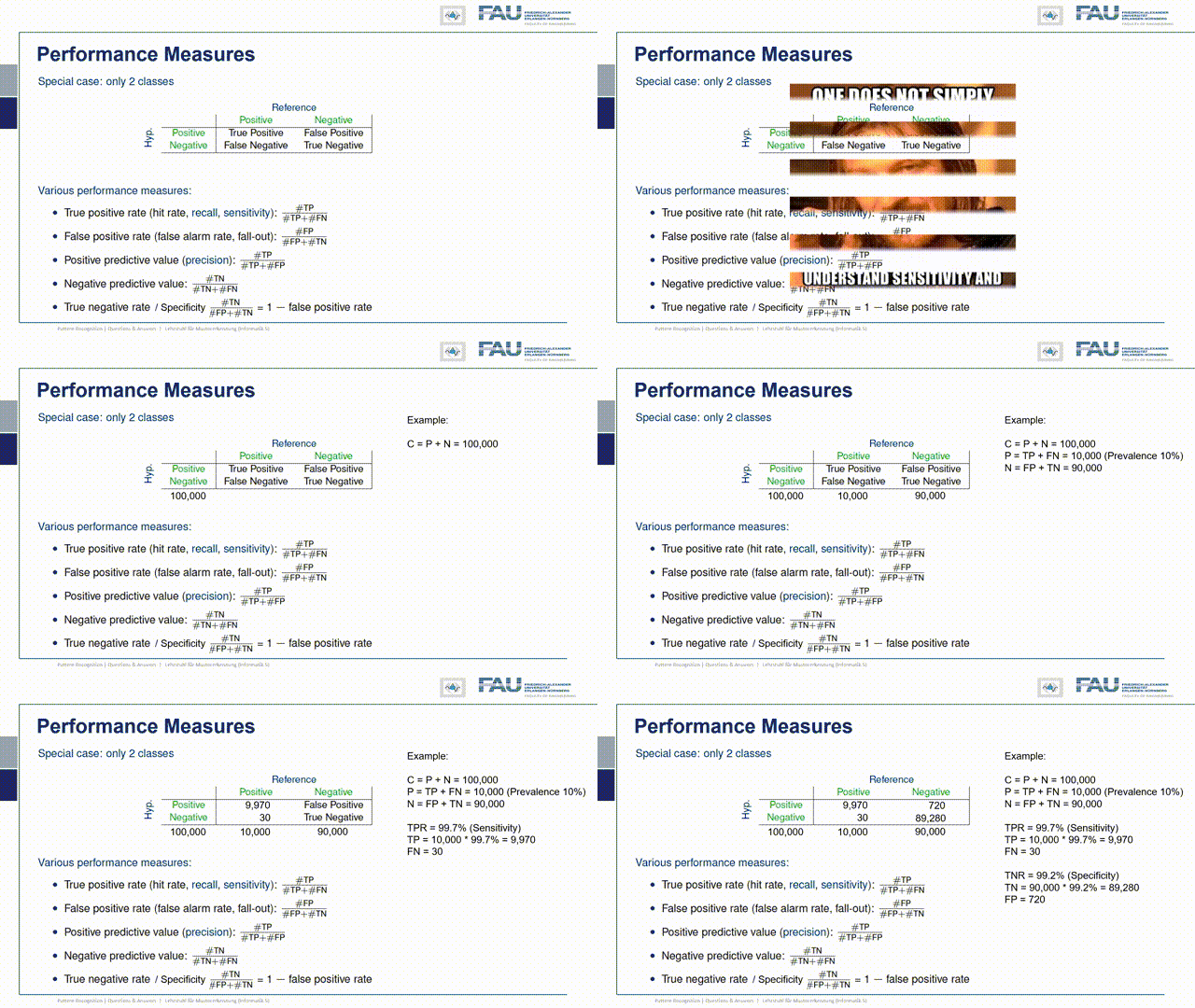
Okay, let’s get back to evaluating our classifier. So the classification system can be evaluated with many many different measures and what you can see here are different means of how to evaluate this classifier. There are of course many different ways how you can combine the above values in order to compute different rates. So a very typical one is known as the true positive rate or also hit rate recall or, sensitivity which is the number of true positives divided by the number of observed positives that is given as the true positives plus the false negatives. Then there is also the false positive rate which is essentially the false alarm rate and this is given as the number of false positives divided by the number of true positives and false negatives. Also highly relevant are measures like the positive predictive value or also precision and the position is given as the number of true positives over the number of true positives plus false positives. Then there is also the negative predictive value which is the number of true negatives divided by the number of two negatives plus false negatives. Last but not least the true negative rate or, specificity and this is calculated as one minus the false positive rate. So this all seems a little bit complex and I’m trying to break these things down a little. So remember one does not simply understand sensitivity and specificity. But I will try to make this easier by going into some examples and the example that I brought to you is the following one. Let’s assume we have a total number of 100,000 people and we will now populate the entire table of examples of these 100,000. We know that 10,000 actually are infected with the zombie disease. So this means the number goes here and another 90,000 have not been infected. So they’re just regular people. So this number would go here in our plot. Now we want to see how good our test is and let’s assume that we know the sensitivity. If we know the sensitivity, we can now actually compute the number of true positives which is the number of positives in our set. Then we multiply with the sensitivity and this yields 9970 true positives and this number then goes here. We can use this now also to compute the number of false negatives which you see here and of course I can also put it in our table. So the other value that is very relevant to determine the actual values in our table is the specificity. The specificity now allows us to compute the number of true negatives which is simply the number of negatives in the reference. So the actual number of true humans and this number is multiplied with the specificity. This then gives us 98,280 and we can put that in our table here. This allows us to compute now the number of false positives which is 720 in this plot. So this value goes here. 

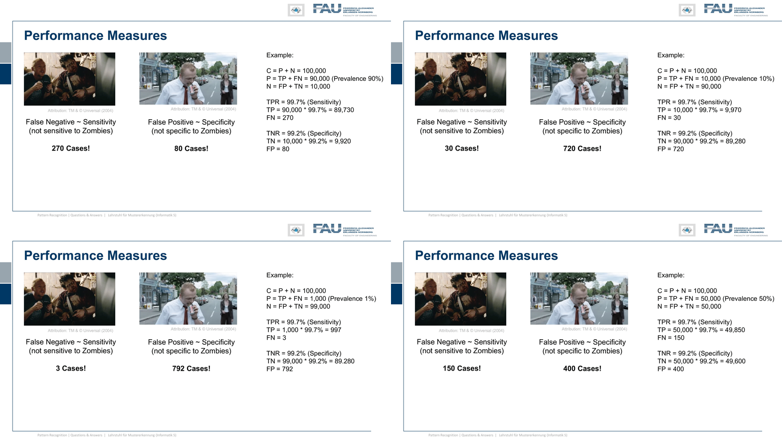
Now let’s think about what this actually means for our test. So you remember our false negatives. This is every time when we don’t detect the zombie. So the false negatives are associated with sensitivity meaning if we have a low sensitivity that means that we are not very sensitive to zombies. So we simply ignore them and think that they are real people. So in this case we would have a total of 30 zombies probably playing video games somewhere or maybe even infecting other people and they are missed by our test. So we couldn’t identify them and we couldn’t take any countermeasures against these zombies because we didn’t detect them. Then there’s also the false positives and you see here in our example the false positives are the hangover guy that just appears like a zombie but isn’t actually a zombie and this is then related to the specificity. So it means a low specificity is related to be not very specific about zombies. So we think people are zombies that aren’t actually zombies. So in our case, that would be 720 people. Now if you are amongst the zombies that are actually not so bad because the zombies will think that you’re one of them and they won’t hurt you. But imagine your fellow humans think you’re a zombie. Well, they might freak out a little bit and you know there could be pretty bad things happening to you. So let’s think a bit about how the prevalence or the prior probability affects our detection rates. Now if we fix sensitivity and specificity then we can see if our prior is only one percent. So let’s say we are in the very very early stage of the disease and then we would basically never find any false negatives. So we would barely ever miss a zombie and the number of zombies is probably so low that people would say there are no zombies out there. So there might be even zombie deniers around that say that these zombies cannot be detected and if you look closely at the cases that have been detected as zombies so there’s very little of them and here in this particular case if we only have 1,000 zombies we still detect something like over 700 people as zombies. So almost half of the detected zombies aren’t actually zombies. Although our test is doing pretty well. So this all might be labeled simply as a myth or fake news or the disease isn’t even out there. So if we gradually increase now the prevalence and we go to a stage where we have 50 percent prevalence. So there’s like half of humanity left and half of humanity is already being converted into zombies you see that our errors change and with the prior we have an increased number of false negatives. So we miss people who are actually infected with the disease and they go and spread the disease further while at the same time we have a reduction in false positives and this is simply related to the fact that there are just fewer negatives around. So the number of false positives is also declining. Let’s say the disease has taken over it has 90 prevalence so in 90 prevalence cases the number of false positives will be greatly diminished, but we have an increasing number of zombies that we are missing but to be honest with 90 or zombies around things are already pretty bad and you may not want to trust anyone. So this is pretty bad in particular a large number of false positives, in the beginning, is very very worrisome.

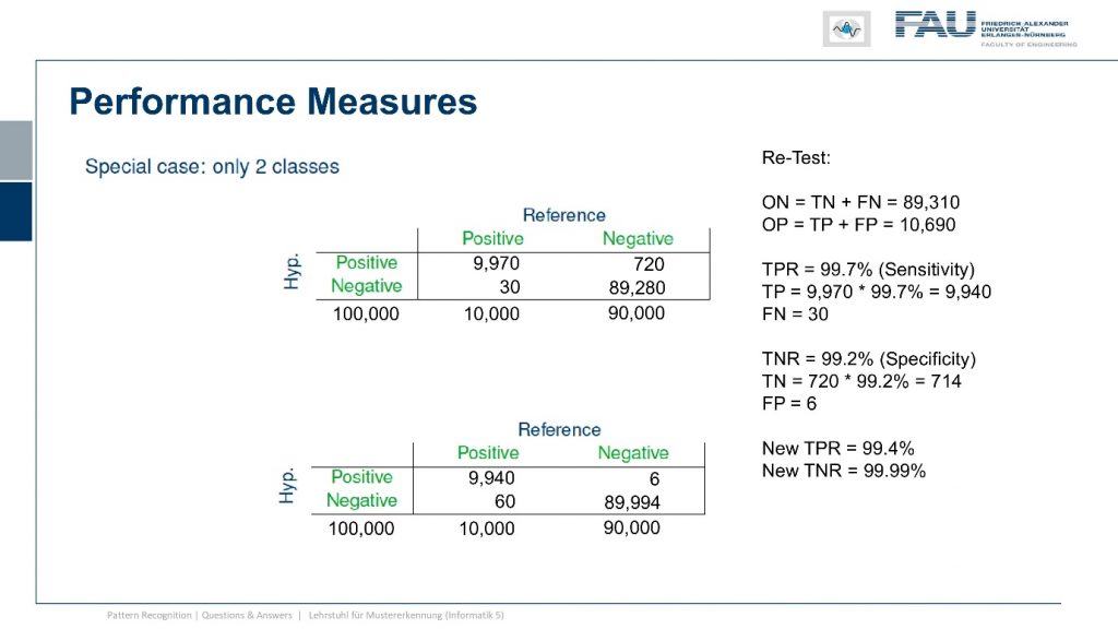
So let’s think about whether we can do something in order to decrease the number of false positives such that we are not harming many hangover people. So if you just have a bad hangover maybe that’s not so great that your fellow neighbors would then decide to use countermeasures against zombies and that could actually be not so great for you. So let’s think a bit about our test we don’t know who the real zombies are we just get the result from the test. But of course, this tells us at least that in the cases where we are positive we may just want to test them again just to be really sure. So what would happen if we do this re-test we just run the same test again, in this case, this is our test result so we have now observed positives and observed negatives and they are only determined by the previous test results. So now we look into the case where we want to retest only the positive cases. So let’s retest those observed positives and in the observed positives are of course true positives and the true positives now we have to multiply with the sensitivity and the sensitivity will then again give us whether it’s a positive or negative result. This means that we retest and a large number of true positives will have another 30 that are assigned to the number of false negatives. Now let’s consider the case of the false positive. So we had 720 we retest them and now we have to consider the specificity. We see now that of the 720 we can identify 714 as false positive. So they will be assigned to negative and this means that we only have six false positives left. So we get a new confusion matrix here. So these are the new results where we already considered the retesting procedure. So you see the number of false negatives has increased to 60 while the number of false positives is reduced to only six. So this means we have a new test in this new testing procedure where we test only the positives twice and it has a reduced true positive rate but it comes at a much better true negative rate. So the false positives are greatly reduced and you see that this number is now much much higher but it comes at the cost of reduced sensitivity. Of course, we could also go in the other direction.

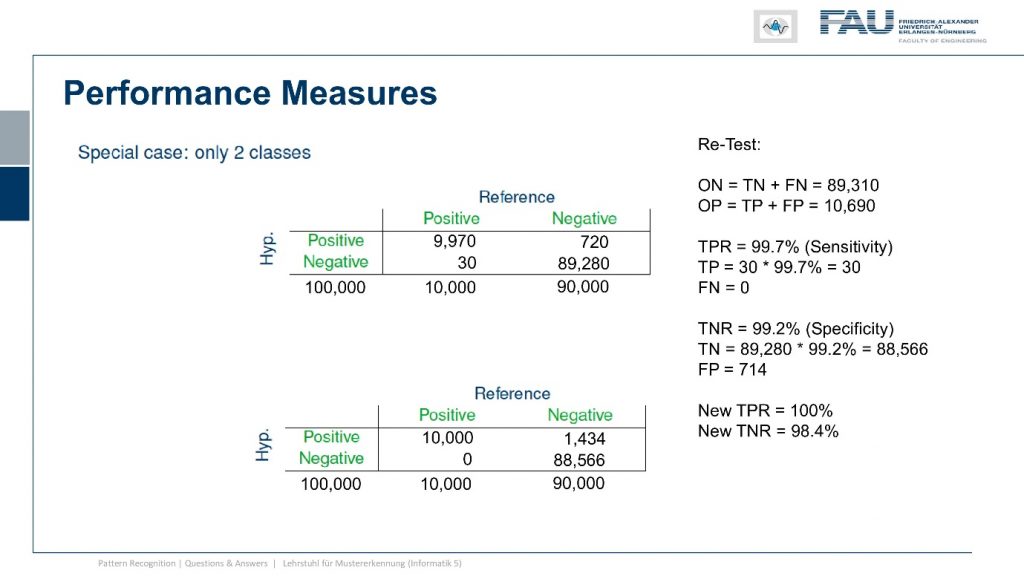
 So we retest only the observed negatives. Now in this case we want to make sure that we don’t miss one of the zombies so we re-test everything that was observed as negative. Now again we have to check our sensitivity and now we see that amongst the observed negatives there were only 30 cases that were false negatives and they multiplied with the sensitivity will now give actually 30 correct classifications. So our false negative number goes to zero. Now let’s consider the other error and we do that with the true negatives that are inside of our set and here we have to use the specificity. We see that we multiply this number and we yield another 714 false positives. So now we can update our confusion matrix which then looks like this one. So we introduced this retesting procedure which gave us a sensitivity of 100 percent. So we didn’t miss a single zombie but it comes at the cost that we now have 1434 false positives. So the number of false positives is almost doubled by introducing this procedure. But we don’t have any false negatives anymore. So remember we only had like ten thousand positives and now we have a thousand four hundred false positives. So this means then that out of the observed eleven thousand four hundred positives there is more than ten percent that weren’t actually zombies. So you’re getting rid of more than a thousand four hundred regular people at the expense of not missing anyone. So you’re taking countermeasures against a thousand four hundred people who have actually not been infected by the disease. So this might be a pretty harsh thing to do and maybe not every government will actually be able to pull this off. Well, we now developed three different testing procedures and now you may wonder are they the same, which one is better, and which one is worse.

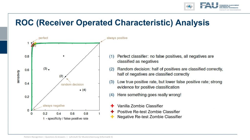
So let’s have a look at them and compare them and the typical tool to do so is the so-called receiver-operated characteristic curve the ROC curve. I’m showing the space where this is evaluating here on the left-hand side you can see in this plot we are plotting the sensitivity over one minus the specificity. You can see a couple of important points on this plot on the top left indicated with the one you see the perfect classifier so this one has a 100 percent specificity and 100 percent sensitivity. So this is always doing the right decision. Another thing you could do is you could simply always decide for positive then you would be at the top right point of the curve and the very opposite is that you always decide for negative then you’re on the bottom left corner of the plot. There is a line connecting those two points and this is essentially a random decision but with varying thresholds. So if you would just roll dice you would be somewhere on the line connecting those two points and this means you do your decision completely uninformed of any observation and this would yield the following line. If you are in the top left triangle you have built a classification system that actually works. So I would expect any working classification system on the top left triangle. So above the diagonal and there’s also the space below the diagonal here indicated by four and if your classifier is located somewhere there it’s more wrong than right. So this means in a two-class system if you will just do the opposite of whatever your classification system is proposing you would actually end up in the top left triangle. So this is the space where we now have to locate our classifiers and we see that our vanilla zombie classifier wasn’t actually doing that bad. It is very close to the top left so it’s very close to the one because it has both very high sensitivity and very high specificity. Now we changed our classification system and re-run all the positives so we changed sensitivity and specificity to yield this point here. So we are slightly moving away from the original classification system and we could improve on the one rate but sacrifice on the other rate. Then we did the exact opposite and we rerun all of the negative cases and then we get this observation here. So we increase on the one rate but decreased on the other rate. So you see that by adjusting the classification system and re-running the decisions I can alter the outcome. Actually, there is a whole continuum of different solutions for sensitivity and specificity and this is shown here by the curve in green and we can essentially move along this green curve with a given classification system. Here you can see this classification system is very very good because it is almost covering an area of close to one. So if I had the perfect classifier then the area under this curve under the green curve would be exactly one and we are very very close to one here. So we have a very good classification system and because it’s the same system that we’re using it needs to be detected by this curve. Now you may wonder how do I get this green curve.

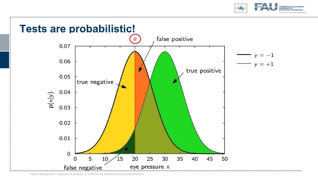
Well actually our classification system stems from two distributions the distributions of the positives and the negatives and determining the actual classification result is simply by picking a threshold on the test statistic. So whatever test do you do? So here in the case of zombies, I hear the eye pressure is a very good measure and while we actually determine whether somebody is a zombie or not you just vary the threshold. So this guy here is important and I can sample the entire green curve simply by varying the threshold. So I wouldn’t have to go through the retesting procedure and running two tests if it’s the same test it won’t change anything because you would simply be adjusting your classifier just according to a different threshold. So that wouldn’t help a lot well what can we do about this.

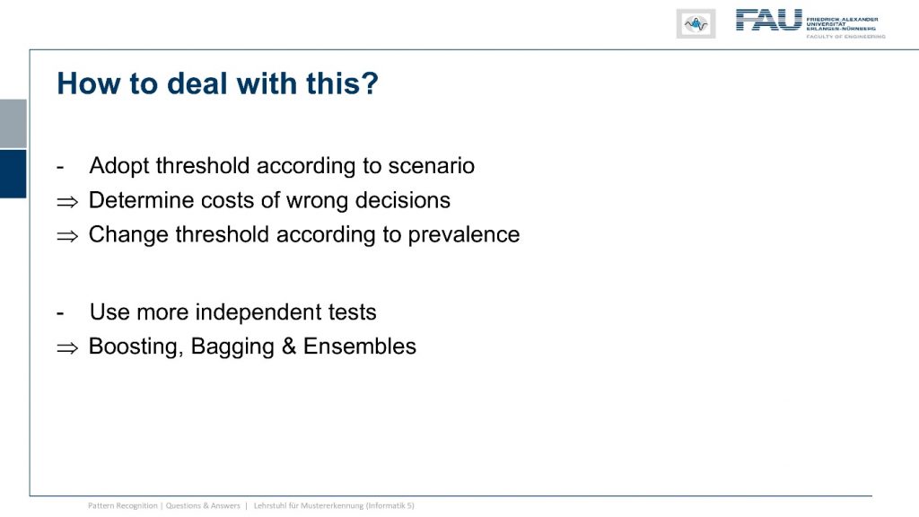
So let’s think about a couple of ideas and one very clear idea is that you pick the threshold according to the scenario. If you want to pick the threshold you have to determine the cost of the decision. So every decision comes with a cost and depending on for example the prevalence of the disease the cost may be very different. So if you are in the early phase you want to stop the zombies at all costs and it would be very expensive to miss one. Because the zombie would just keep on spreading the disease. In later phases of the disease, this may be very different. So probably you want to adjust your threshold according to the current testing scenario and you can do that if you know the cost for the decision because that allows you to weigh what is more costly, the false positive or the false negative. Another idea is to involve another test and you just test with two different tests and if they’re statistically independent you can combine the two in order to get a better decision. This then leads to concepts like boosting bagging and ensemble classifiers that we also will talk about in this class. Now one thing that I want to give you in order to understand these ensembling properties is what I want to show you a specific example.

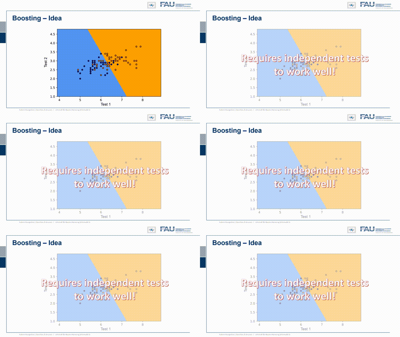
So what you typically do is you then run a second test statistic and with the second test statistic, you can then create plots like this one and then find a decision boundary that is orthogonal to one of the two tests. This means that you can harness the power of the two tests. Whenever we do boosting and ensembling we typically assume that the tests are statistically independent. So this is a key ingredient and let’s look at an example where this is the case.

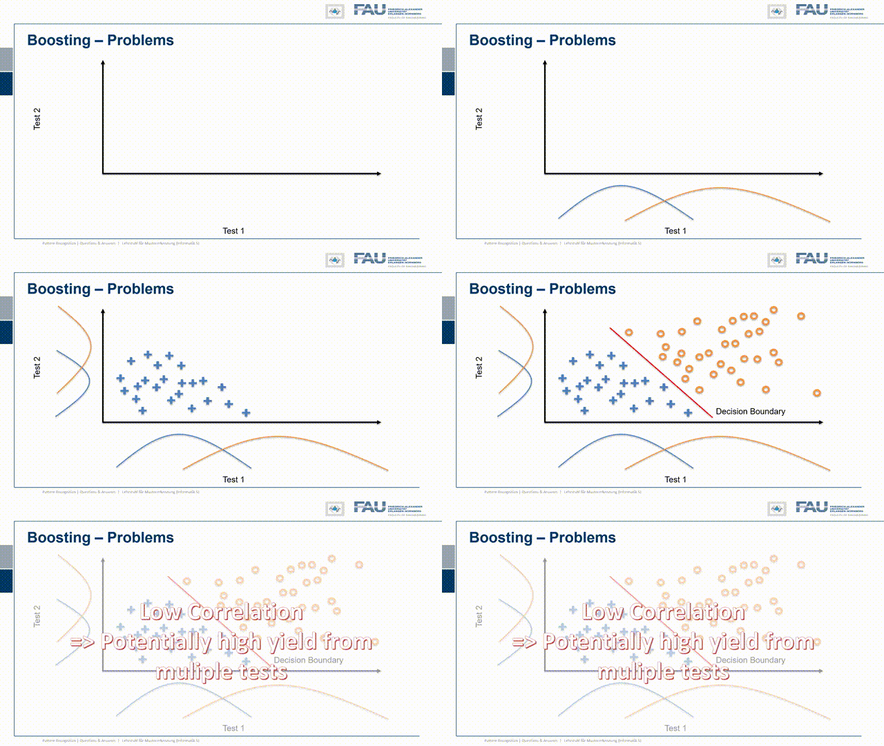
So I have test statistic 1 and our class 1 and class 2 or positive and negative are distributed in the following way. So there’s a significant overlap. So they both are somehow not separating the classes very well and I have another test where of course the same two classes are appearing again. Now I want to combine the two and now let’s pick a configuration of observations and these are now indicated as the true class and the true other class, so the positives and negatives. Here you can see that I essentially have to find points that follow the projection on the x and y-axis onto the original distribution. I did that here in this case and you can see in this particular case the distribution of points follows the respective one-dimensional projection. So if I just move them to the one side or to the other side and by the combination of the two tests I can get this very clear separation here. So this is very useful and in this case, we really have the independence of the two tests and because they are independent there is potentially a very high yield of combining them. 

Now let’s look at an example where the classes are much better separated and here I have one class the other class now the overlap is very small. I do the same on the other axis and the overlap is again very small. This then means that the blue dots have to be distributed somewhere where they get projected onto the blue curve and the orange dots have to be located somewhere that they get projected onto the orange curve. This is a bit problematic because you see how we are very close to the diagonal and actually we have a correlation of test one and test two. So the two results are not completely independent and whenever I have this kind of very good separation already and the assumption that these are Gaussian distribution points on the test statistic, then I run into this problem. The problem is now that because the two tests are correlated there is very little yield by combining the two. So you see here a decision boundary. It’s a bit better but it doesn’t solve the problem as neatly as we’ve seen in the previous case. So if the two are correlated it’s much harder to piece the two tests out of another and to benefit essentially from the other test statistic because they are almost measuring the same thing.

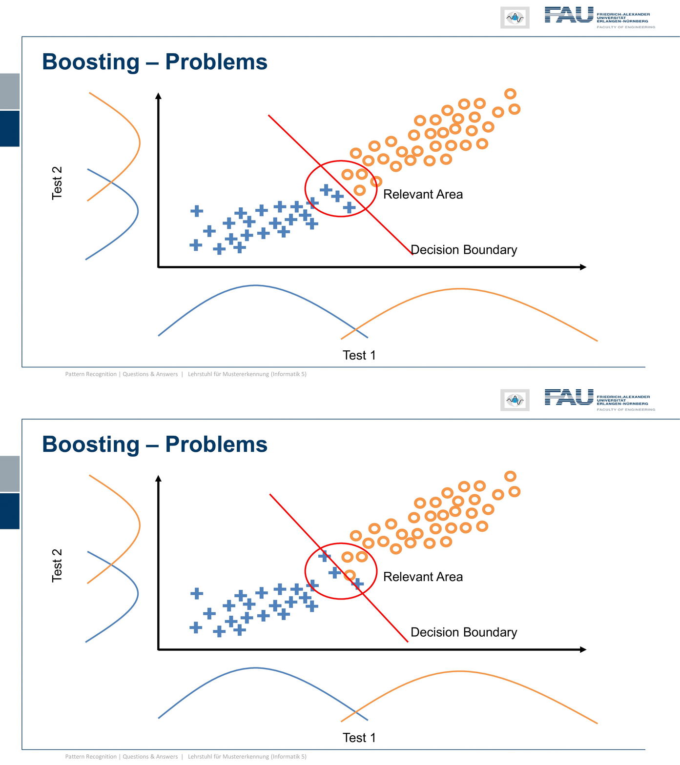
Now of course this doesn’t mean that it’s impossible. So what is relevant is this area here and if I’m lucky with the tests then I can find a configuration that solves the problem much better. But of course, only the small area where the two classes are actually connected is the area where I can get yield. This is very hard to describe with the statistics only on one of the two axes so you really have to know the complete distribution of the classes and their joint probability distribution otherwise you won’t be able to determine this so easily. Well, I think these were quite interesting observations and gave you a little bit of insight into evaluating classifier’s test statistics and also what the sensitivity and specificity of a classification system also have in terms of implications.

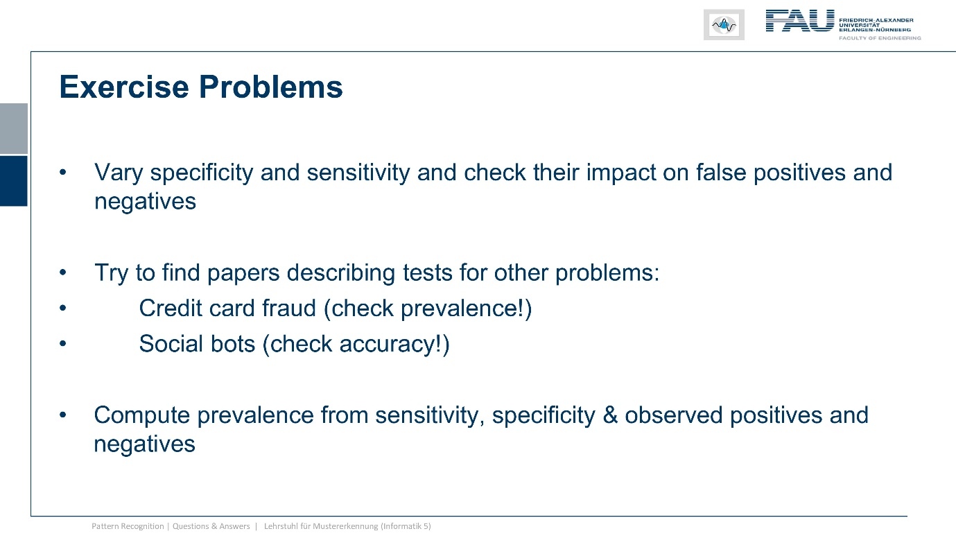
I prepared an additional set of exercise problems that you can think about in order to even gain a deeper understanding of what I’ve shown in this video. In particular, you should think about varying the sensitivity and the specificity and think about how this would change the number of false positives and false negatives. Also, I think it would be interesting to screen literature and look for sensitivity and specificity reported in papers for example on other diseases. So this can help you to understand how relevant the classifier is how many false positives and so on you would get and I would also recommend checking the prevalences of different diseases because some diseases are very prevalent and then you have a very different implication for the false positives and false negatives than in diseases that are occurring at a different rate. So two examples that I have here check credit card fraud and you will see that it’s very rare that fraud actually occurs. So imagine what that implies on the requirements for the false-positive rates and then also check the literature on social bots which are also very interesting because then the accuracy of the classifier is extremely low. Then you can think about what this probably means about the bots that have been found and reported in the studies and yeah you will see that this is actually a pretty interesting phenomenon. If you have a really bad classifier I mean it will of course always identify social bots but does it really help you to figure out that this person is really a social bot or not is mass screening with such a poor accuracy really a very meaningful thing to do? Well think about it yourself and then another very interesting problem is to compute the actual prevalence if you know the sensitivity and the specificity of the test and you have the observed number of positives and negatives. So this is also something you can think about in an exercise problem. So this brings us already to the end of this unit.

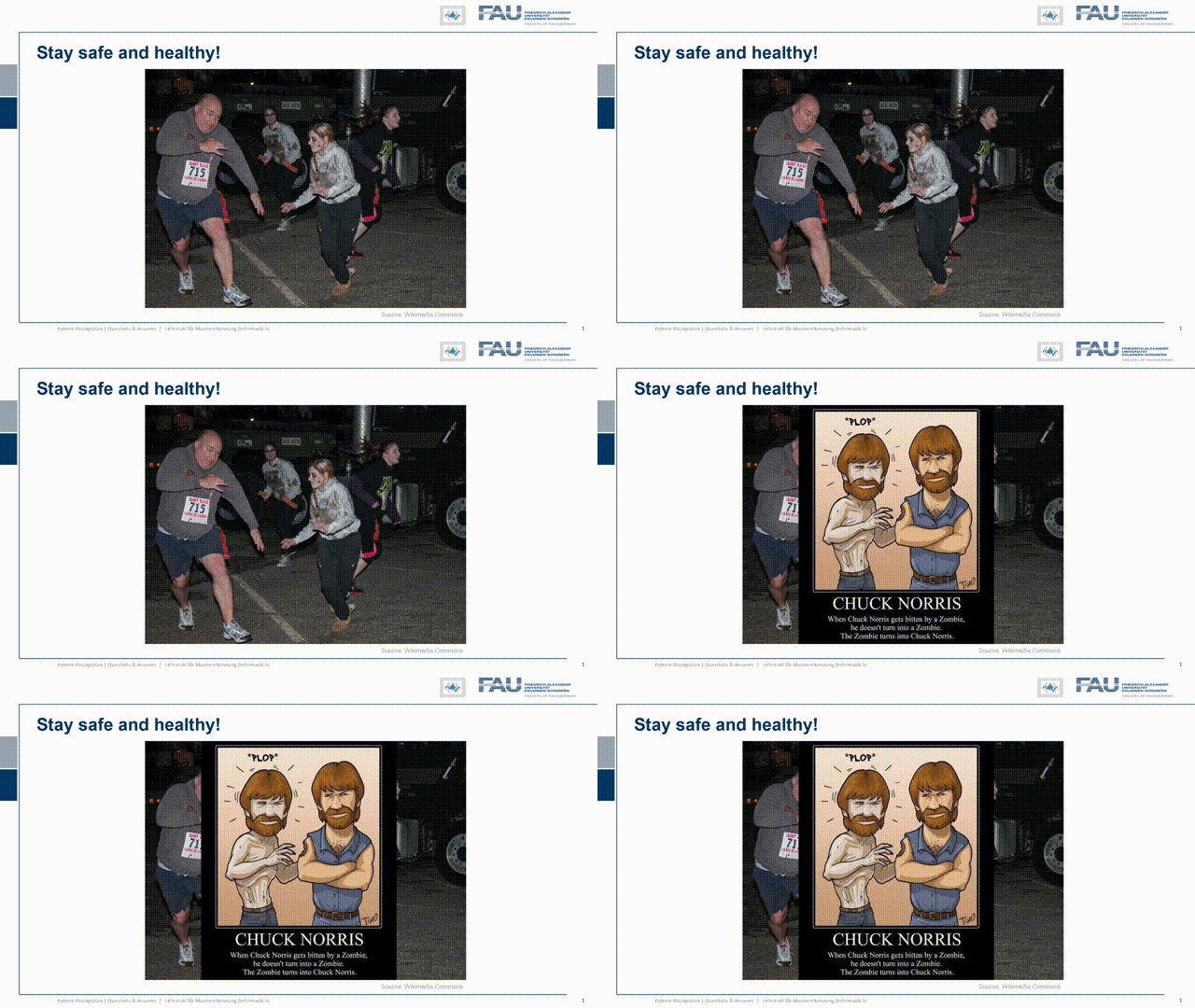
So stay healthy keep away from zombies and yeah I don’t want to leave you without some hope. Remember if chuck Norris is ever bitten by a zombie struck Norris won’t turn into a zombie but the zombie will turn into chuck Norris. So here are some contact details if you want to follow up and watch more videos. 

So I think I also have a couple of other interesting things about pattern recognition and machine learning here. This already brings us to the end of this video I hope you had some fun watching this and you understood a little bit better about sensitivity and specificity, what this means, how this is related to false negatives and false positives and how large the implications can actually be if you do anything wrong with this regard. So thank you very much for watching and looking forward to seeing you again in one of the other videos. Bye-bye!!

If you liked this post, you can find more essays here, more educational material on Machine Learning here, or have a look at our Deep Learning Lecture. I would also appreciate a follow on YouTube, Twitter, Facebook, or LinkedIn in case you want to be informed about more essays, videos, and research in the future. This article is released under the Creative Commons 4.0 Attribution License and can be reprinted and modified if referenced. If you are interested in generating transcripts from video lectures try AutoBlog

Category: Lecture Notes in Pattern Recognition