Lecture Notes in Pattern Recognition: Optimization Primer

These are the lecture notes for FAU’s YouTube Lecture “Pattern Recognition“. This is a full transcript of the lecture video & matching slides. We hope, you enjoy this as much as the videos. Of course, this transcript was created with deep learning techniques largely automatically and only minor manual modifications were performed. Try it yourself! If you spot mistakes, please let us know!

Welcome back to our pattern recognition Q & A. I’ve received again many of your questions and I selected a couple of those to be replied to in this video and today’s video will be all about convex optimization, Lagrangian mechanisms, Lagrange formulations, and things concepts like strong duality. I picked a couple of very simple examples which I hope will help you understand those rather mathematical concepts. So looking forward to discussing some examples for convex optimization, Lagrangian optimization regularization, and strong duality. 

Okay so I prepared this small set of slides and I summarized some of your questions and then again we are talking about pattern recognition, machine learning. You know it can always get worse imagine that you would be dealing with things like described in this book here. So don’t worry about it we’ll get there and I’m making these Q & A videos such that you can understand the mathematics that we’re discussing here in much better detail.

So again popular questions. Something that occurs quite frequently is emails like this one.

I want to work in your lab, pretty pretty please do you have a job. Can you give me a Ph.D. topic? Can you supervise me? Can you hire me and so on. Unfortunately, it’s rather hard to find a job in tech and it’s not like that we don’t have any applications or something like this. 

So it’s pretty competitive to find a good position and you know one does not simply find a job.

But what if I told you that we can actually help you with finding a position.

So we actually have quite a few social media groups and in particular, on LinkedIn and Facebook we regularly post also job offers there. Not only with us but also with our partners. 

So if you’re looking for a job or, Ph.D. position, we publish those things always in our social media groups. So don’t send just your cv to me but you can join the groups I will post the links here in the description of this video. We are publishing positions for assistant jobs at our university, for Ph.D. positions, for postdoc positions and we even have sometimes positions for professors not just in our group but really in our network collaborators all around the world. We will post them there and you are of course welcome to join those groups. If you find something that you think is a good match then send your cv and don’t take the effort of just sending CVs out there to everybody. It’s not very likely that we will have a position that is not advertised in this group. 

So if Nick Cage can still get work then you can do anything. Keep that in mind okay.

So let’s go to the actual topic. We want to discuss a bit what convex optimization is and why it’s important. You know this is a convex function here y equals x square. The cool thing about this is if we do a minimization here doesn’t matter if we start here, follow the negative gradient direction we end up here. But if we were to initialize here we would follow the gradient direction and we would still get the same minimum. So that’s the cool thing about convex optimization and doesn’t matter how you initialize, you will end up with a global minimum. So this is why many people like to do convex optimization and try to find mechanisms how you can actually formulate a specific problem convex and then you get these very nice solutions.

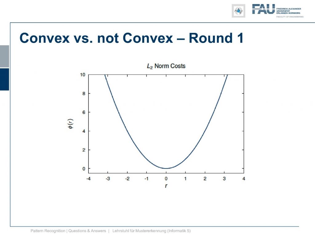
Now I prepared a few quizzes for you. What’re convex functions and what are not. So let’s do round one convex versus not convex. Round one this function well you’ve probably seen it before. I’ll give you some time to answer………..

The answer is yes. This is a convex function. Okay so let’s go ahead round two convex versus not convex.

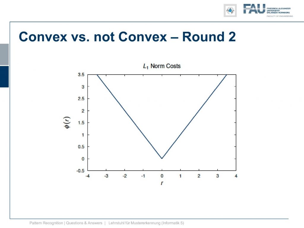
The L1 norm. Now, what do you think? Is it a convex function? Remember convexity you connect two points of the plot and they always lie above the function and you look in detail.

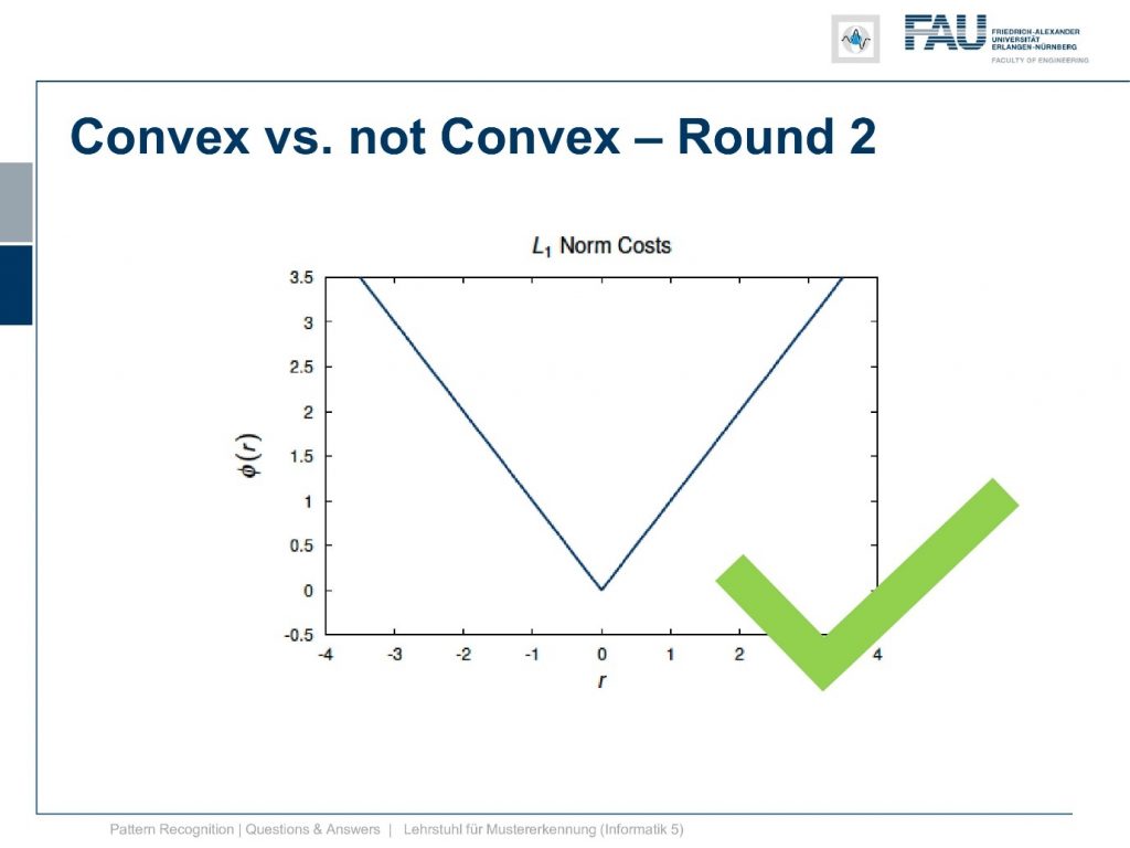
It is convex again. Actually, we had quite a few of those penalty functions, and those penalty functions that I’m showing here, all of them are also convex.

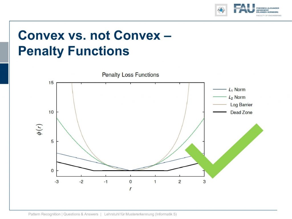
So these will help you also in finding convex optimization problems. If you like to use those norms that are actually quite helpful. So also those are convex. Let’s go into round three and here we have another penalty function that we discussed.

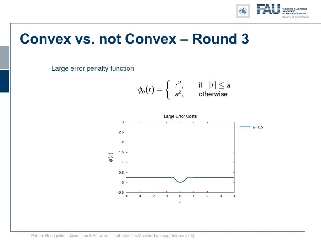
This is the large error penalty function and here you see that we are actually cutting off at a certain large error and assign a constant loss.

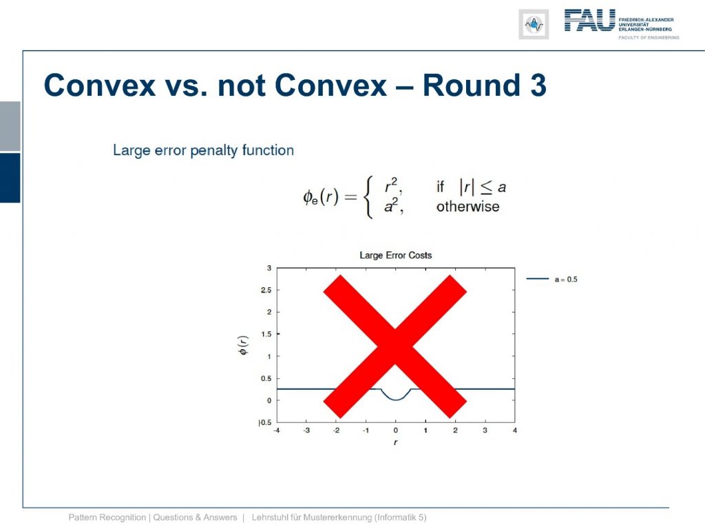
This one is not convex and why is it not convex? 

Well, of course, we can find points that we connect and they lie above the function, but of course there are points also like these two if I connect them we are lying below the function. So this is not a convex function. 

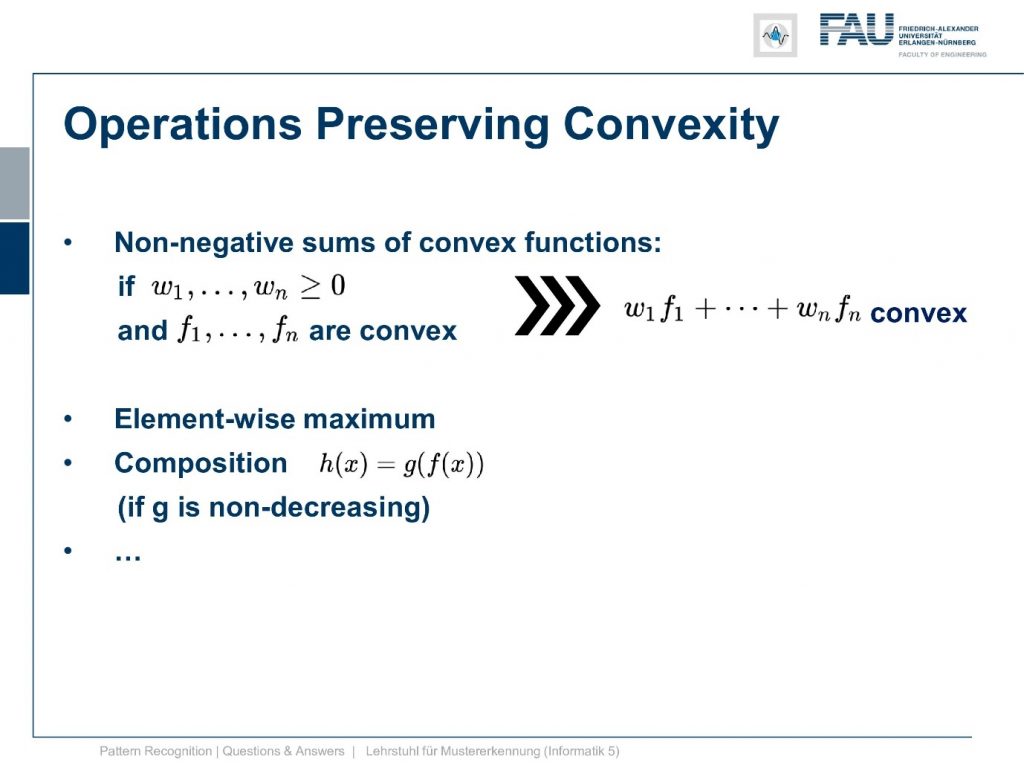
So convexity is quite cool and it can also be preserved. So there’s also a couple of operations that conserve convexity. This is for example the non-negative sum of convex functions. So if you have positive weights and you have some set of convex functions, then if you have a weighted sum of them this is also convex. So this is useful element-wise maximum is also a convex function and also a composition saying that you apply one function of another function can also be a convex combination. But this is here only the case if g is non-decreasing. There’s a couple of more variants of this and you can find them in your favorite math textbook about convexity. We are not essentially writing up all of the possibilities of preserving convexity, but I just wanted to name these couple of examples here because they are relevant for our class. 

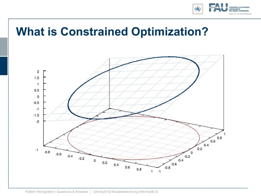
Also, you were very interested in constrained optimization and constrained optimization we had this example in the class that we have. Let’s say a plane and then you want to find the point that maximizes the plane given that it’s on this circle. This example seems straightforward but it’s again already a little bit complex. Because if we go into the Lagrangian formulation we end up with a three-dimensional construct and this is harder to visualize. So I decided to come up with an even simpler example and this is the one that I want to discuss today.

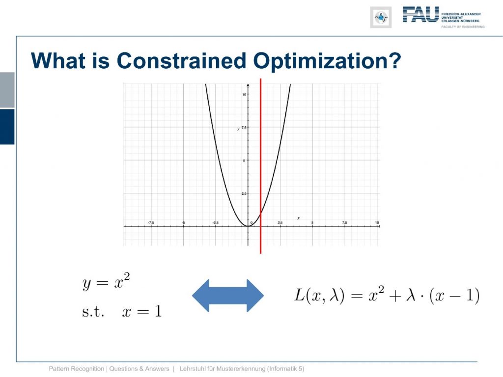
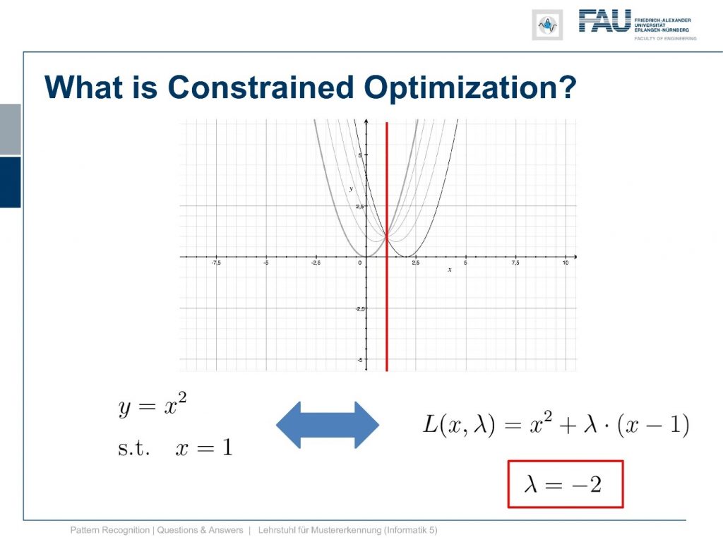
It is simply y equals x squared and now I also need a constraint. So it can’t be a 2d constraint but we have a 1d function so it’s a 1d constraint and it’s subject to x equals 1. So this is super easy because now the solution is x equals 1. After all, there is no other solution and x equals 1 right. Well, this is of course an academic example and I want to show you how the Lagrangian then looks like and so on and how we can deal with this constraint. So this is the position that we want to find with the kind of constrained optimization and we can already indicate it here in this graph. 

Now how can we find this and Lagrange tells us that we can set up a Lagrangian formulation here. We introduce a Lagrange multiplier λ. 

Now you see that we multiply the constraint the zero constraint actually just with λ and added to the original function. So we end up with L(x,λ). So we now have a two-dimensional function and this is given by x and λ. The Lagrangian is then simply the sum that is weighted with the Lagrange multiplier as we give the constraint to this. Now you see if you compute the derivative with respect to λ you can immediately see that everything that is related to the original function will cancel out and only the constraint will be preserved in a critical point meaning the position where λ equals to 0 is a position where the constraint is fulfilled. So this is one of the main ideas of the Lagrange multipliers.

Let’s have a look at how this function behaves with different λs. So if we start with λ=0 you can see we just have the original function the constraint is gone. So this is simply the original function. Now let’s play with λ a bit and I’m choosing here  -1, -2, -3, -4 and you see by choosing different λs we change the function and the function now is shifting up and down. So this is interesting isn’t it and you can see the position where we have the peak is exactly the position where our constraint is fulfilled. 

So this is kind of interesting. so let’s think about this a little more.

So we want to find a solution for Lagrangian and what we just see is that for λ=-2 we seem to have found a solution. So for λ minus 2 the minimum of our lagrangian is exactly the desired minimum where our constraint is fulfilled. so this seems to be an interesting function. Let’s look at a 2d plot of this function and here you can see how it actually behaves. 

You see on this axis that we have essentially a parabola that is smeared over the λ domain. so we have different variants of this parabola and you can see that there is a critical point here a saddle point where we go up and then down again. So we are looking for critical points in the Lagrangian because these are related to the solutions of our constrained optimization. So it’s not necessarily an extreme but it’s a critical point that we are interested in. This critical point is essentially found here with λ=-2. Okay, so you see that this is also not a bounded function. So if you simply do a gradient descent procedure here you will not find the correct solution. This is even not bounded with respect to λ. So you need a constraint minimization toolbox and for example, interior points methods in order to solve this. So it’s not just that we have a solution here where we just minimize and do gradient descent and get the right solution. We need to be able to get the critical point so that’s the thing here. 

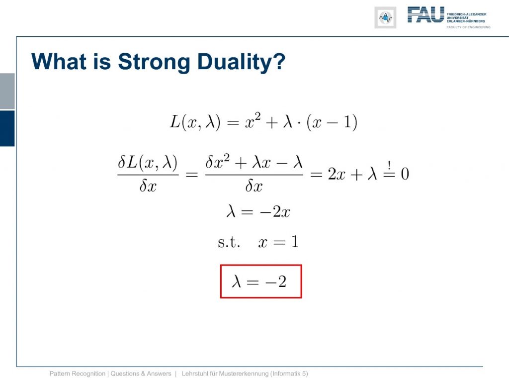
Now we can also have a look into the idea of strong duality. In order to do so, we compute the partial derivative of our Lagrangian with respect to x. Here if you look at this one you can see that we need to change it a little bit. We multiply the λ into the bracket and then you see it’s very easy to actually compute the partial derivative with respect to x. So this is simply 2x plus λ. Now, this is supposed to be a critical point and this critical point is of course a position where this is equal to zero. So we can set it to zero and then we can solve for λ. Now if we look at this then we can see that our constraint was x equals to 1 and this results exactly in λ equals to -2. So this is already the right thing but we were actually looking for the dual.

So this didn’t give us the dual. So let’s think about this again.

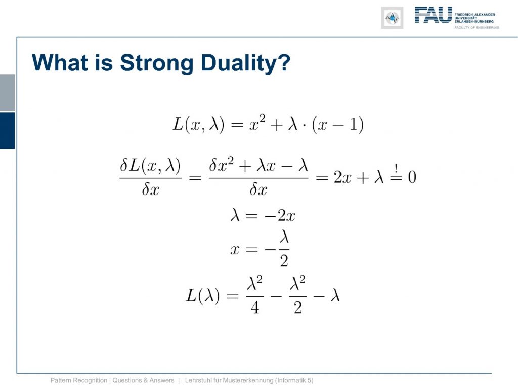
Now we again have λ equals to minus 2x. Now we solve for x and you see that by solving for x we get x equals to minus λ over 2. This is also a very nice feature because we already know that λ is minus 2 now. If you plug it in here you see the solution for λ gives us also the solution in x. So we see that we get x equals 1. We can take this now and plug it in into our lagrangian function and get the dual. Now you see that our dual is λ squared divided by 4 minus λ square divided by 2 so we can simplify this further. So this gives us then minus λ to the power of 2 divided by 4 minus λ. 

This is interesting because now we have a function that only is dependent on λ and x has canceled out completely. So let’s have a look at this function and plot it here. 

So this was our original or primal and this is now our dual. Now, this is actually a strong duality. It’s a strong duality because the infimum over the primary is found exactly at the position where we also find the solution to our primal problem. So you see here we have a zero duality gap, they both lie on the same line so there is no difference between the solution of the primal and the solution of the dual. So the duality gap is zero. 

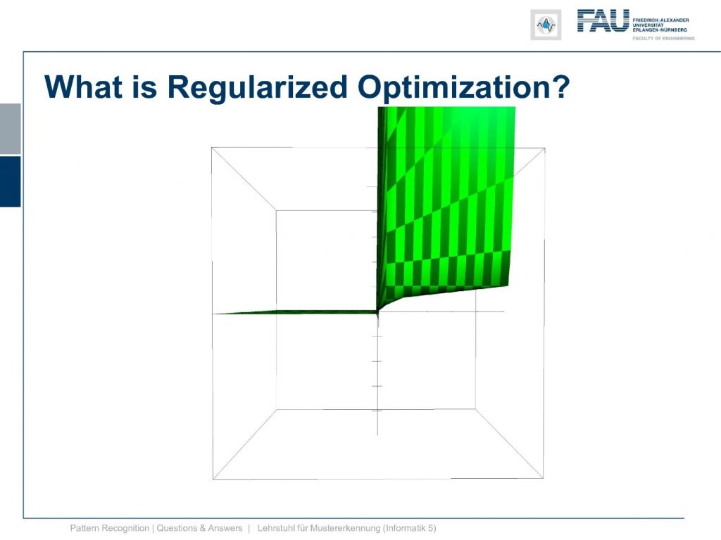
That’s actually pretty interesting but given that we could already solve that x equals one, we can feel now like a boss because we have solved the quadratic function using strong duality. You had more questions and another question was what is regularized optimization?

Now here you have a solution to a regression problem here on the left-hand side and typically you have many observations and you want to solve it and you can do it with what we discussed in our video about classification and regression. Now regularization you need when you have cases like this one. So you have just one observation and you want to fit a line. Well, then you end up with the problem that it’s not unique. The regularization can now help you with finding the correct line because for example, you could constrain your slope to one and then you would probably end up with the solution yeah. So regularization can help you in those ill post problems where you have trouble finding the correct solution. You use prior knowledge on the slope in order to get it in there. 

So you don’t have to break your head we can help you with regularization. 

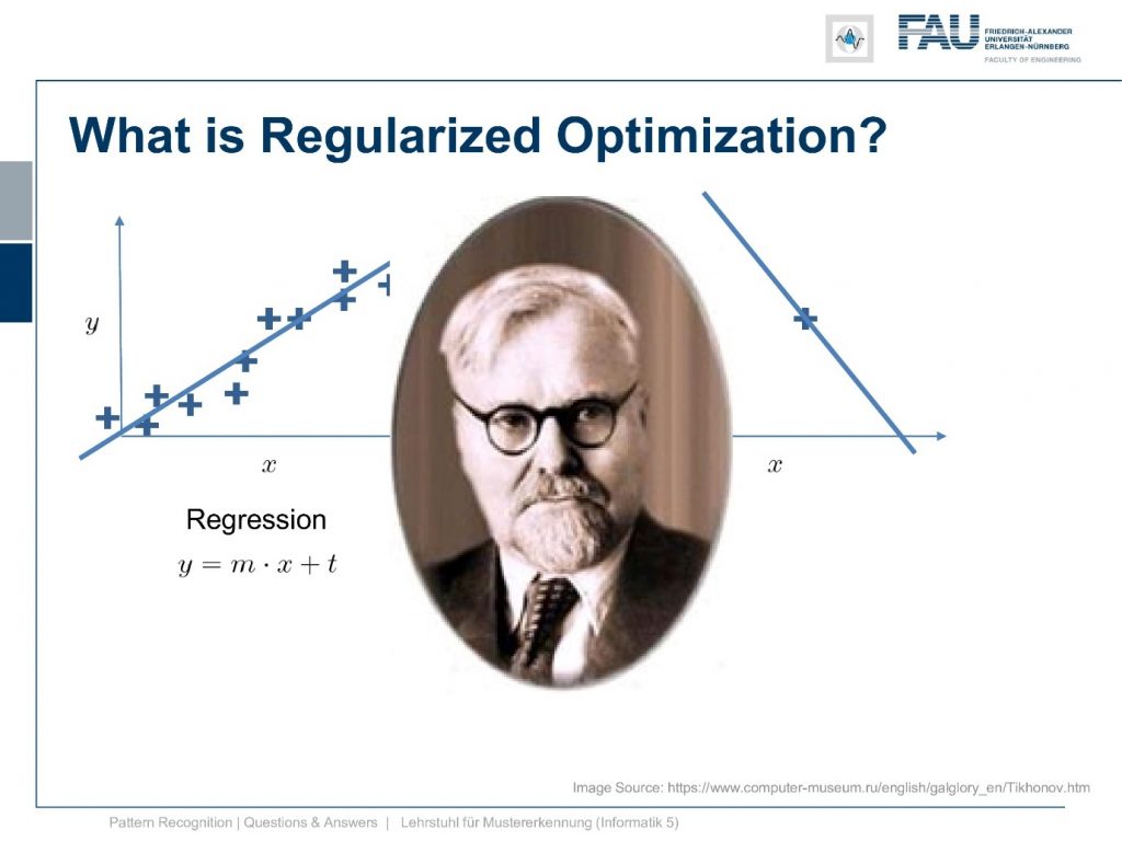
This is where our friend Tikhonov comes in. He has proposed a particular kind of regularization and it’s very useful to embed priors into our regression. So how can we do that? 

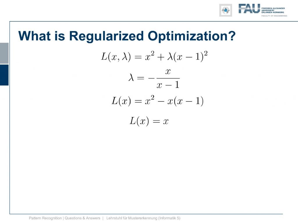
Well the thing is we have again our primary function that is y equals to x square and again we need to embed a constraint. Here again, the constraint x equals to 1 but we express it now in terms of a distance. So we say the difference between x and 1 to the power of 2 is equal to 0. So we use a quadratic constraint here and of course, this is a power of 2 but you can generally also do this with two norms on vectors and so on. But we are only using a 1d space here so it’s simply the square but generally, you can also use two norms for ticking off regularization. If you use the L1 norm then you end up with the lasso. So this doesn’t matter that much right now but you see that we have an equality constraint and how do we deal with equality constraints? Well, we use our good old friend Lagrange and we are multiplying it again with a Lagrangian multiplier into our lagrangian function. So here now the lagrangian is given as L(x,λ). So again the dimensionality increases and then x squared plus λ times x minus 1 to the power of 2. 

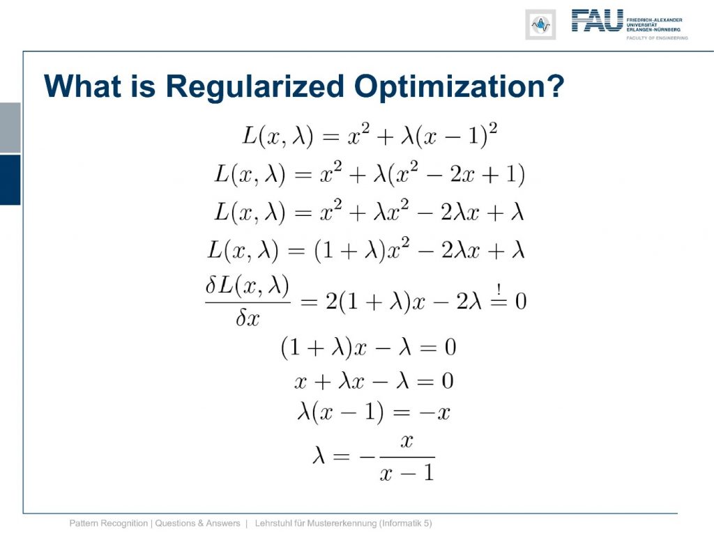
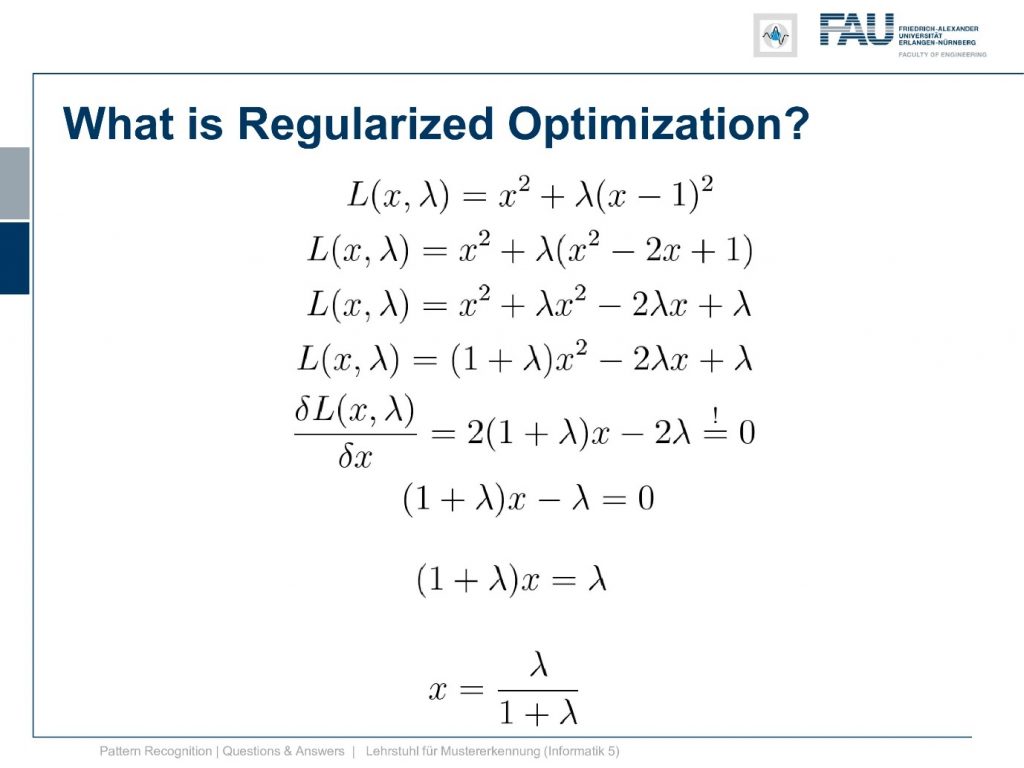
Okay so let’s have a look at this function. Again we rearrange it a bit so first of all we get rid of the square and you see that we can express the square bracket using this term here. We want to compute the derivative with respect to x again this is why we multiply in the λ and then we can simplify this a bit so we can pull out the one plus λ and just have one term of x square one term of x and one term without any x. Now we compute the derivative with respect to x and you see that this then gives us two times one plus λ times x minus two λ. As we already learned in the first part of this video this needs to be zero because otherwise, it wouldn’t be a critical point. So we can set it to zero then we can divide by two and end up with this statement here 1 plus λ x minus λ equal to 0. so we can still reformulate the bracket. So we take x plus λ x minus λ equals 0. Now we can bring over the minus x and divide by x minus 1 and you see that this is our solution for λ and let’s look at this in a little bit more detail.

Remember this is subject to x equals to one. Now let’s plug this in and we see we have to divide by zero.

So what kind of a problem is this? Why is this actually a good thing to do? Okay let’s think about this a little more.

Now that we have a solution for λ. We can also plug it in into a lagrangian and try to find a solution for the problem without any λs and only with x’s. If we do so you see λ only appears once. So we plug it in then the sign flips the divided by x minus 1 falls out. We can essentially get rid of the power of 2 on the right-hand side. Then this gives us this function here. Let’s think about this a little more multiply the x into the bracket and we see that the x to the power 2 cancels out and everything that remains is x. 

Now, this is also not nice because if we want to minimize this problem or maximize it it’s not bounded. It goes all the way to minus infinity and plus infinity. So it doesn’t help us either. Well, let’s look into the dual.

For the dual, we can go back here and then we solve for x instead of λ. So we bring λ to the other side and we divide by 1 plus λ and this is our solution for x. Now with the solution for x, we can think about this and oh yeah if we have the solution to x we can build the dual.

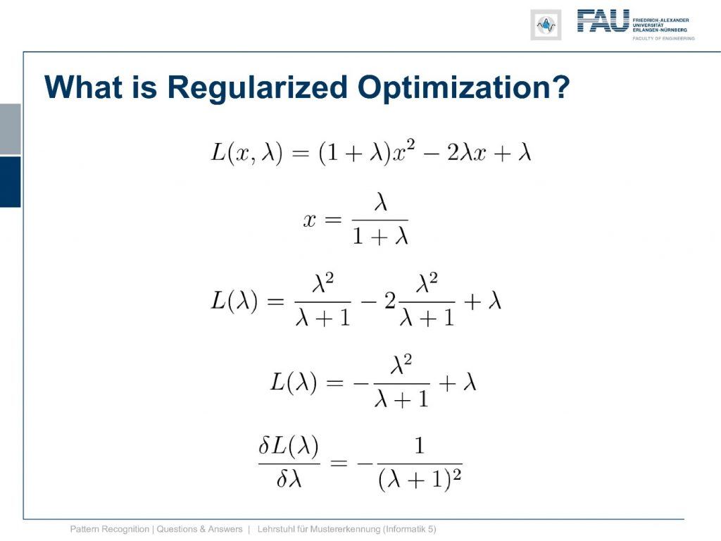
So we take now this version here of the lagrangian that we encountered as one of the steps. So this is a very nice version because we already have only one power of two of x and only one x in there. So we can take our solution for x and plug it in and you see again we have the bracket canceling out. So we have λ to the power of two divided by λ plus one. Then the same term again but with minus two and plus λ. So this cancels out once. So we have minus λ to the power of 2 divided by λ plus 1 plus λ. Now we’re interested in solving for λ. So we find the derivative of this guy with respect to λ and if you rearrange this a little bit you find this is minus 1 over λ plus 1 to the power of 2. So this is the derivative of our dual and we need to set this to 0.

Now let’s think about this a little bit.

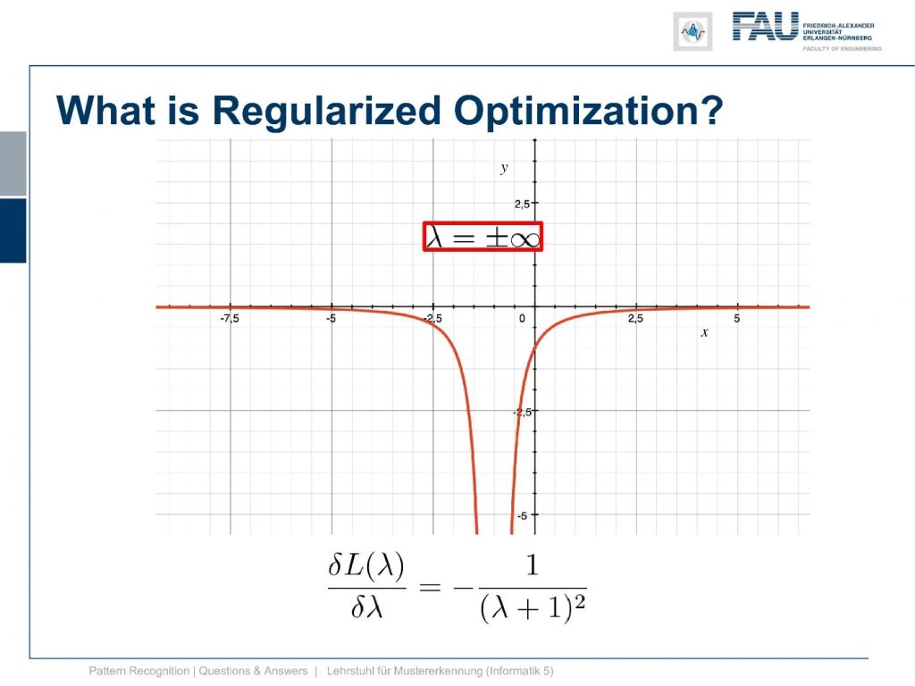
Let’s look at the plot of this function you see that this guy only approaches zero at plus and minus infinity. So what the hell is this? How does it help us to solve this problem?

Well, let’s go back to our original problem, and let’s just play a bit with the values of λ.

 So let’s look at the shapes that we take if we are changing λ and now we start with λ zero again then the zero we have the original solution. Now let’s gradually increase λ and you see with increasing λ we get functions that gradually approach having the minimum exactly at the desired location. 

Then let’s have a look at the solution for the lagrangian with respect to x. Now you see this is lagrangian of x equals to x and this is this line and you see that all of the minima that we have found with different versions of λ. They all lie on this line. So this is already something that is kind of useful to understand what you’re optimizing for and you can also see that I have to essentially scale up λ towards infinity to exactly reach the solution where we have fulfilled the constraint.

Okay well, let’s look in the other direction. Now, what’s happening if we are choosing negative λs and if you see if we have already minus 0.5. We already get this parabola and at minus point eight we get this and at minus point nine, we already get this. So, this goes down very very quickly and we kind of have a function where the minimum goes down further and further and it’s going completely in the wrong direction. So, this is absolutely not what we want to have and already at λ equals to 1 we get a line. So here the quadratic term cancels out completely and we get this line, by the way, intersects our other Lagrangian. The Lagrangian of x exactly at the solution which we can see here. but now if we look at our dual you see that at λ minus 1 our dual is going towards negative infinity and then right after -1 we are coming back again from positive infinity. So, we have a huge jump in there because we are dividing by λ and we have this kind of hyperbole that we have to deal with. So, this is the position where we then degenerate into a line, and here you can see then that we can go ahead towards the solution on the other side so we can go below -1 in λ. This might be interesting so let’s look at what’s happening here so let’s try λ minus 2.

Now you see we’re coming in essentially from the other side suddenly and with decreasing negative λ you see we kind of also approach the position x equals one. So we get to the solution x equals one. This however is no longer a minimization problem but a maximization problem. So we flip the parabola entirely and then we suddenly approach the solution from the other side. So minus negative infinity is also giving us the right solution. But this is entirely not how we thought that this would behave. So this is probably not the way that we want to go after. So the solution is really at plus infinity for λ and minus infinity for λ.

We said the solutions in our Lagrangian, they must be critical points of the Lagrangian and remember this is a necessary but not a sufficient condition. But now we can have a look at this graph and you now understand why the change in λ is causing this upside-down flipping of the parabola. If you want to reach positions where the gradient approaches zero in both directions then of course you have to go plus minus infinity with λ otherwise you won’t find such a position. So, this is a very interesting way of visualizing this and you may not understand anything in this plot if we hadn’t looked at the examples earlier to understand what we are actually doing here. Okay, so our regularization kind of works but not exactly as we intended to do it right.

So actually it might be a much better idea to restrict our problem only to have positive λs. What now happens is if we restrict λ to be positive we are essentially going into a constrained optimization with inequality constraints. So in inequality constraints, you force the Lagrangian multiplier to have a specific sign. Here we require the λ to be positive. Now, what would happen if we introduce this if we look at the dual so the orange curve in this plot all of this will be gone. So all of the negative values will no longer be actual feasible values. So they are not part of the optimization, they are not feasible points in our problem so we can neglect those. You see that if we neglect those only the parabolas that I’m showing here are remaining so only the positive λ parabolas are remaining and these would then be part of the Lagrangian that we seek to optimize. 

So still our solution is plus infinity here to get the exact fulfillment of the constraint and to be honest we probably want this constraint to be exactly fulfilled. But if we wanted to be exactly fulfilled we now have convex constraints and a convex primary. So this means that we have a strong dual problem again. So this is strong convexity and you can see here our duality gap is exactly zero. So you see that here again this line duality gap zero. This is exactly where we approach the solution. So this is pretty cool and if you are attending our lecture you will also find the concept of slater’s conditions and if you have convex functions and convex inequality constraints then slater’s conditions hold and we have strong duality. 

Now let’s have a look at the kind of 2d surface plot that emerges here. 

So we now get rid of all the negative parts. So I set it to 0 here for the visualization and you see that this is the kind of lagrangian that we seek to optimize. Again the solution here is at positive infinity. Maybe we don’t want to have this constraint completely fulfilled.

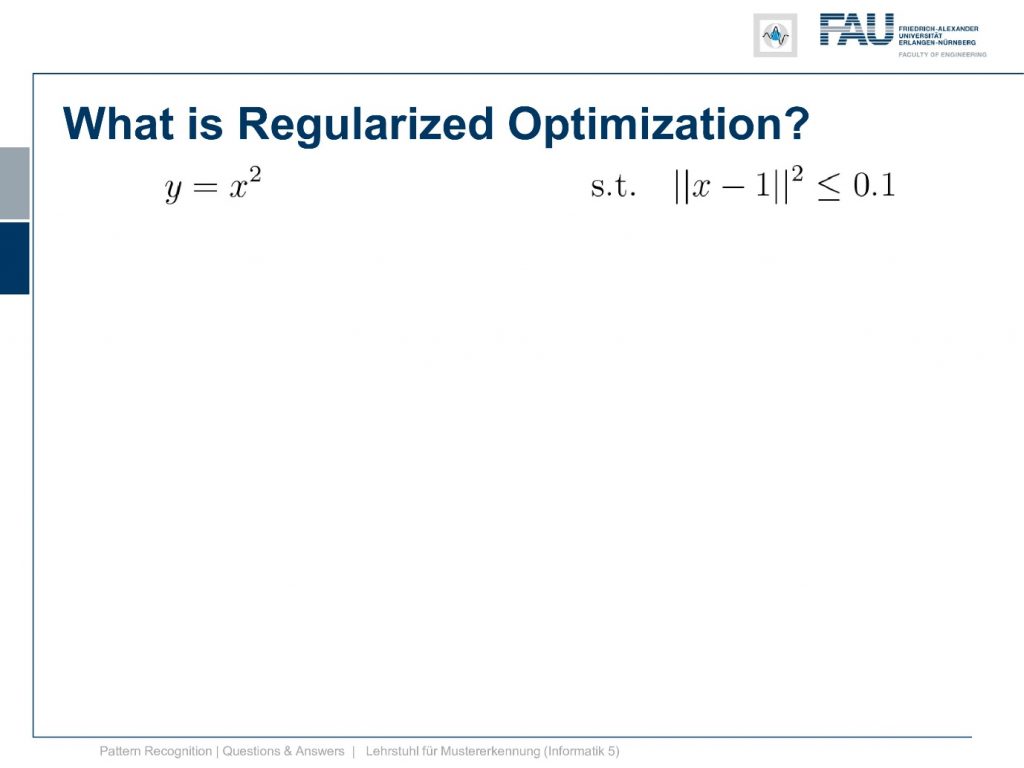
So why does it have to be zero? How about setting the constraint to be below 0.1. 

So we want to have a small norm. We don’t want it to be exactly zero but we want to have it below 0.1 and then we can set this again up to constraint that is to zero you set up lagrangian and so on. 

If you do that you suddenly get this kind of function as the solution and now you see because we introduced this kind of parameter it could be an epsilon here the point zero one. You see that our curve doesn’t increase anymore. So there is a λ at which the condition is fulfilled. So if we are less away than point one we have a feasible solution and then we also have a gradient that is zero everywhere. So we have a critical point. So you could set some epsilon that is larger than zero and force the inequality to be in this kind of fashion. You then realize that setting this epsilon is essentially the same as setting a specific λ that is positive enough to have the constraint fulfilled. This then gives rise to this whole chain of argument why many people then say okay the Lagrange multipliers. They are just engineering constants and you set them to a sufficient number and it’s correct. Actually, if you set the Lagrange multiplier to a specific value you implicitly choosing this epsilon. But you would have to do the math to actually determine the epsilon value instead you can just set the λ to a fixed value and then you remember you have a convex combination of a convex constrained and original convex function. So in this kind of domain, you’re then even dealing with a convex optimization problem and you can go ahead and just do gradient descent. So this brings us back to convexity and why regularization can help us setting up convex problems.

So you could argue a little bit that regularized optimization is a little bit like in this figure here. So you engineer the parameters just to be able to find a good solution. 

So remember math is your friend and math will always be there for you even if there is no one left on earth. So I hope you enjoyed this little video I thank you for your attention. 

If you have more questions just go ahead and ask them using the comment functionality, using the different ways of interacting with us in forums that we have for FAU students but also on social media on different platforms. I’d be happy to take your question if they’re related to the stuff that I’m actually talking about in the video and not about things that are completely wild like solving your homework problems and so on. So these questions I won’t answer. But if you’re interested in this class and you have questions and they require a little more to actually be answered I might even be inclined to make another video like this one. So thank you very much for watching if you liked the video then I would be very much looking forward to welcoming you again to another of this question and answer videos but for sure I’ll be producing also other lecture videos. So stay tuned. Bye-bye!!

If you liked this post, you can find more essays here, more educational material on Machine Learning here, or have a look at our Deep Learning Lecture. I would also appreciate a follow on YouTube, Twitter, Facebook, or LinkedIn in case you want to be informed about more essays, videos, and research in the future. This article is released under the Creative Commons 4.0 Attribution License and can be reprinted and modified if referenced. If you are interested in generating transcripts from video lectures try AutoBlog

Category: Lecture Notes in Pattern Recognition