These are the lecture notes for FAU’s YouTube Lecture “Pattern Recognition“. This is a full transcript of the lecture video & matching slides. We hope, you enjoy this as much as the videos. Of course, this transcript was created with deep learning techniques largely automatically and only minor manual modifications were performed. Try it yourself! If you spot mistakes, please let us know!
Welcome back to Pattern Recognition! Today we want to continue talking about the Logistic Function. Today’s plan is to look into an example of how to use the Logistic Function with a probability density function.
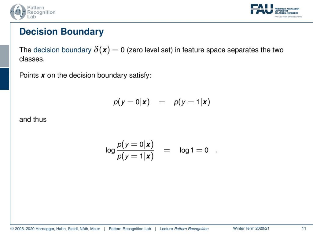
So this is our decision boundary that can be modeled with the Logistic Function. Let’s say our decision boundary δ(x) equals zero, so this is the zero level set. Now we can see that the zero level set can be related to the Logistic Function. So points on the decision boundary will satisfy exactly that the two probabilities, meaning the probability of class 0 and the probability of class 1, are equal. So this is the point of equilibrium. And this is essentially the place where we can’t decide whether it’s the one class or the other. Both of them are equally likely. Then we can rearrange the fraction of the two in the following way: We apply the logarithm to the fraction of the two posteriors and this is then the logarithm of 1. And the logarithm of 1 should be equal to zero.
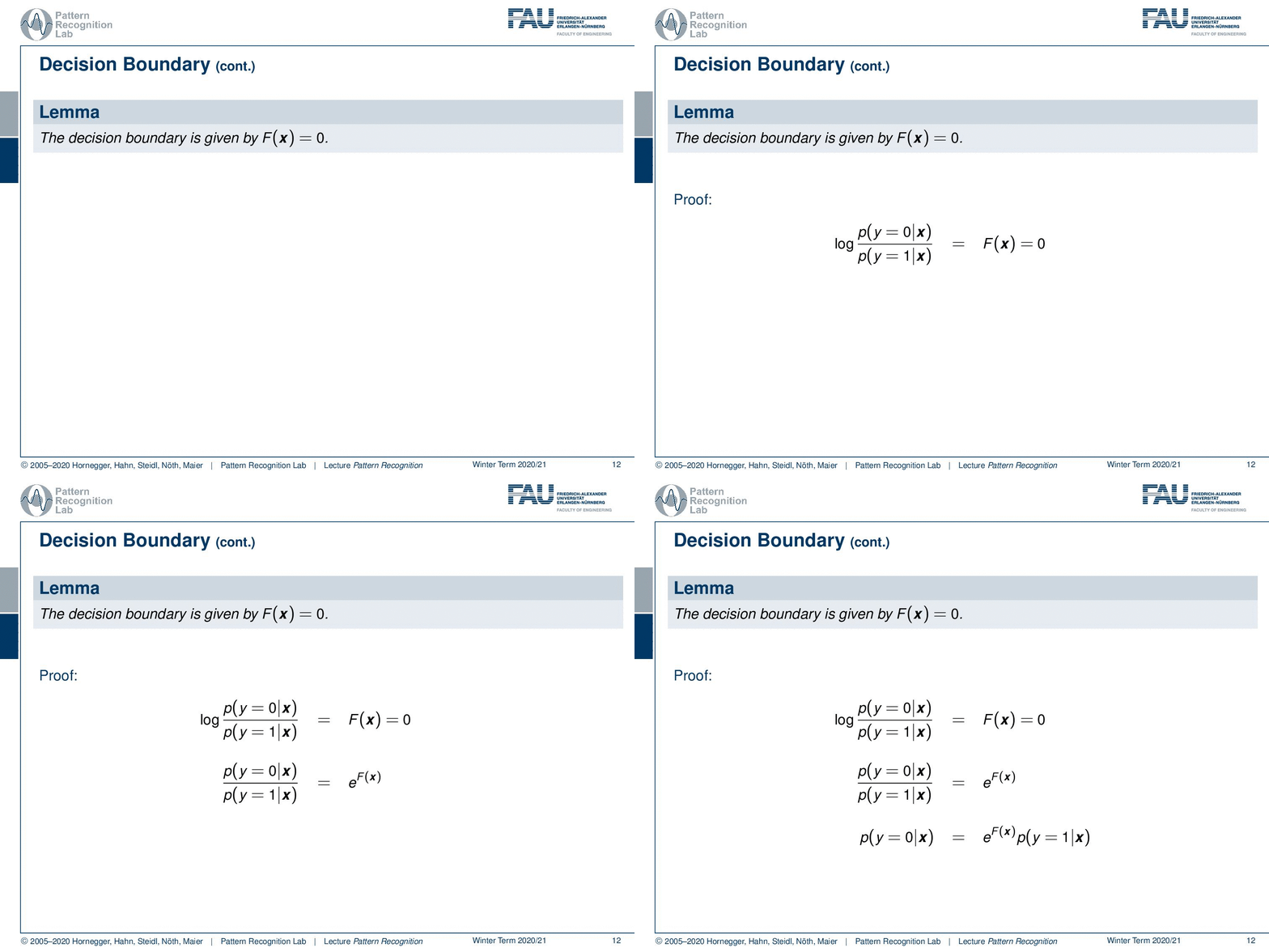
Now we can state that the decision boundary is given by F(x)=0. Let’s look into the proof. Here you can see that we apply the logarithm to our posterior probabilities. This is supposed to be F(x)=0. We can then of course apply e to the power. This will cancel the logarithm on the left-hand side and we get eᶠ⁽ˣ⁾ on the right-hand side. Furthermore, we can now rearrange to p(y=0|x). So this is actually the probability for our class 0. And we can see that this can be expressed by the respective term here on the right-hand side.
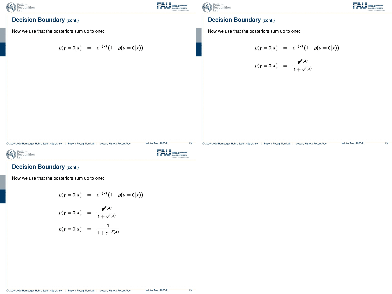
Now the probability of y equals to 1 can be expressed in our case also with the probability of 1 minus the probability of y equals to 0 given x. So this is a slight modification here. And now we can see that we have 2 times p(y=0|x). We can actually rearrange this. This gives us then the following solution. Now you see we are already pretty close to our logistic function. And we can rearrange this simply by dividing everything by eF(x). And then you see that the only thing that remains is 1 over 1 plus e-F(x). This is nothing else than our logistic function.
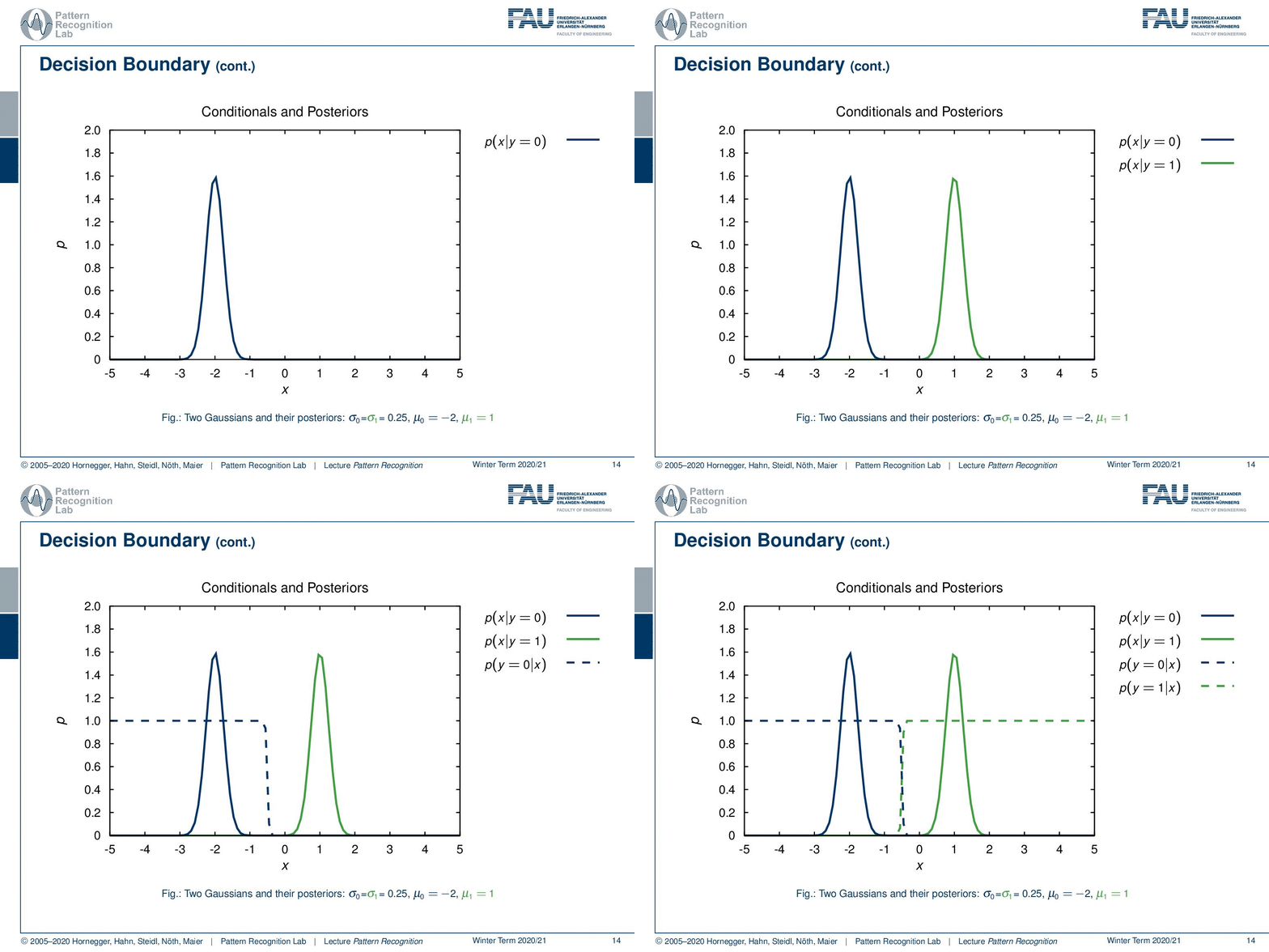
Let’s have a look at some examples using a probability density function. Here you see the probability of x given y equals zero. Of course, we can also find the probability for the opposite class here. You see that we have two Gaussians. The Gaussians simply have the same standard deviation and the means are apart. Now we can also find the posterior probabilities. So you see that the probability for y equals 0 given x is indicated here by this dashed line and for the opposite class, we can find it as this dashed line.
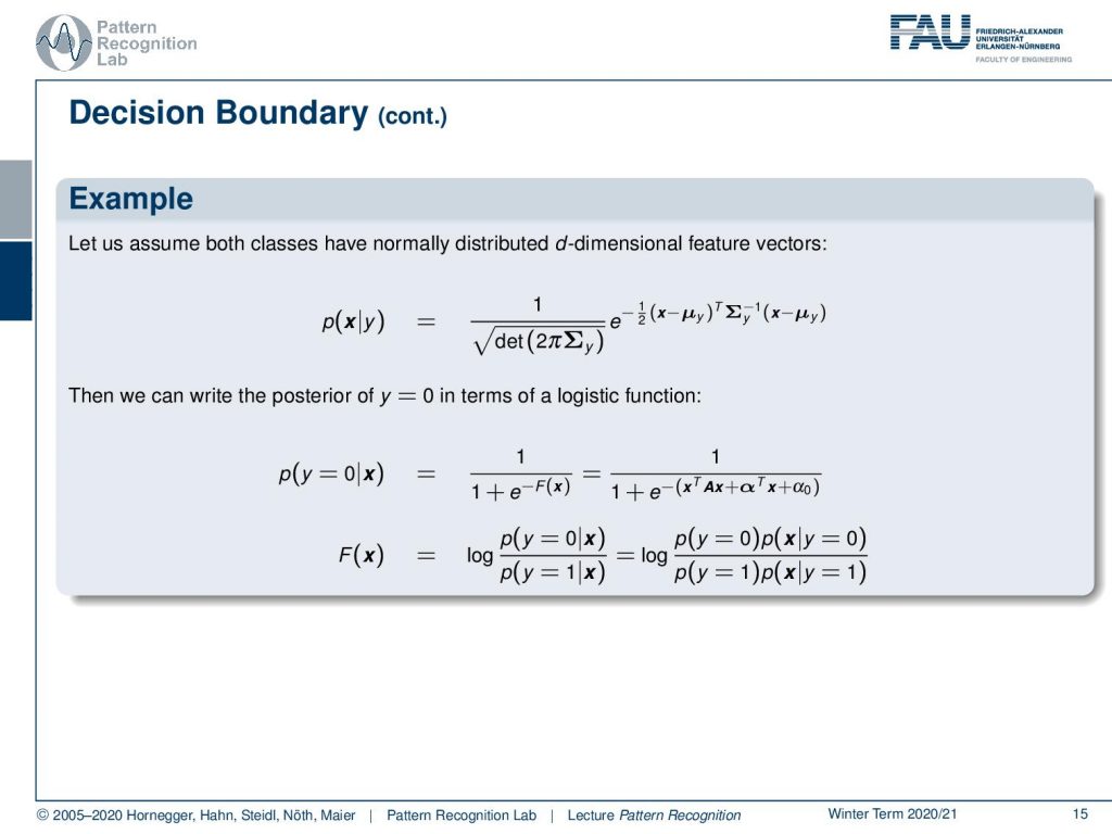
Now let’s go ahead and look into an example. Here, our example is a multivariate Gaussian that is given this probability. So, we can see this is the standard where we introduce a covariance matrix that is given as Σ and a mean vector μ. Now we want to show in the following that the entire formulation above can, of course, also be rewritten into a posterior probability. Here then we want to find the Logistic Function. This Logistic Function then should be expressible in the right-hand term. And here you see that we essentially have a quadratic function in x. This quadratic function can describe exactly the posterior probability if we have two different Gaussian functions. Now let’s try to find the solution. What we’re interested in is finding the decision boundary F(x). And again, we use the trick that we want to rewrite it in terms of the generative probabilities. So we write it here as the priors times the probability of x given the respective classes, and we put that in a kind of fraction.
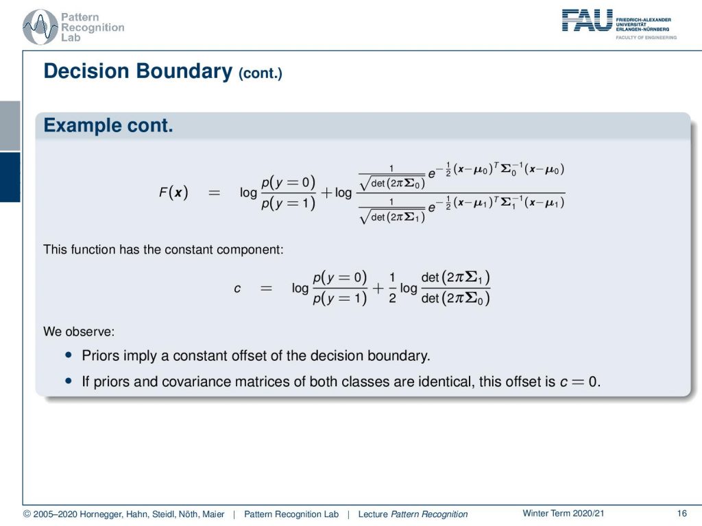
If we do that, we plug in the definition of the Gaussian. And you can see we did this on the slide. So we essentially have the fraction of the priors, and we have the fraction of the Gaussian. You see that we have μ₀ and we have some covariance Σ₀ as well as some μ₁ and Σ₁ for the second class. What we can already figure out if we look at this term is that there are quite a few things that are not dependent on x. So we can pull out a couple of things from the above equation. All the things that are not dependent on x are essentially the priors and again the scaling variables in front of the Gaussian distribution. You can see here, that essentially the covariance matrices and the priors give us a constant component that is a kind of offset. So we observe that priors imply a constant offset to the decision boundary. And if the priors and covariance matrix of both classes are identical you see that this offset is simply 0. So if we have two times the same prior probability, then the first term in c will cancel out and will be 0 because the fraction here will be 1. The same thing will also be true for the second part where also the fraction will be 1, and then the logarithm of 1 will be 0. So this is also an interesting observation.
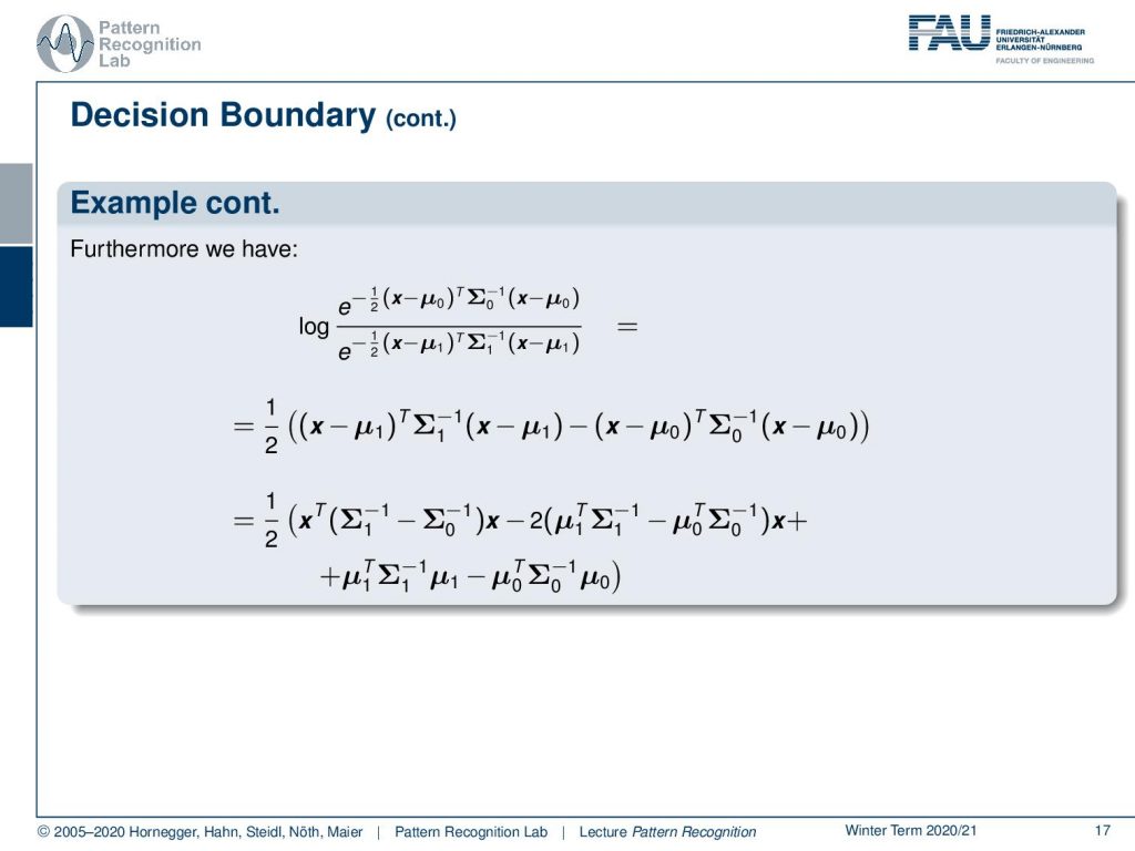
What else? Well, we can also look into the remaining part that is dependent on x. The part dependent on x we can also reformulate a little bit because the logarithm can be used to get rid of the exponential functions. And if we do so, we can rewrite this essentially into these terms that you see here. These are essentially the terms that are used in the Gaussian in the exponent. Now you see that these are kind of quadratic terms that are going around the covariance matrices. We can reformulate this a little bit by multiplying out all of the terms. You see that we can find essentially a description where we have the quadratic term. Then we have a linear term, and we have a term that is simply a constant that is no longer dependent on x.
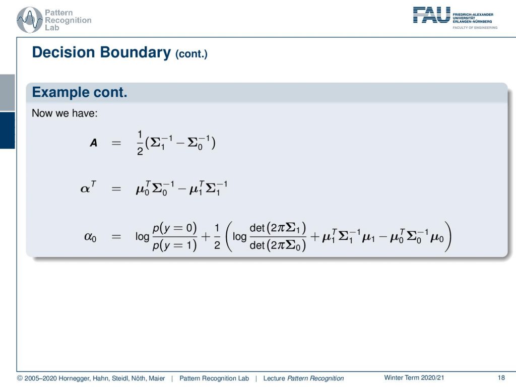
Now we can rearrange this and map it to our original definition that we wanted to use for our decision boundary. This gives us now the matrix A that is constructed from the two covariance matrices. Then we have this vector αᵀ. αᵀ is constructed from the means, multiplied by the inverse covariance matrices. And we have some α₀ that is essentially composed of the constant term c that we’ve seen earlier, plus the additional constant term that we have derived on the previous slide. So it’s very nice that we can essentially find the decision boundary of the essential intersection of two Gaussians always as this kind of quadratic problem.
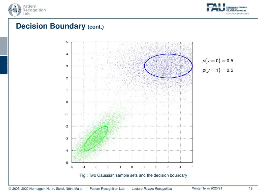
Now let’s look at a couple of examples. So we have two different Gaussian functions here. We have a blue and a green one. You see that they have the same prior in this configuration. We also indicate the covariance matrices with the ellipses here.
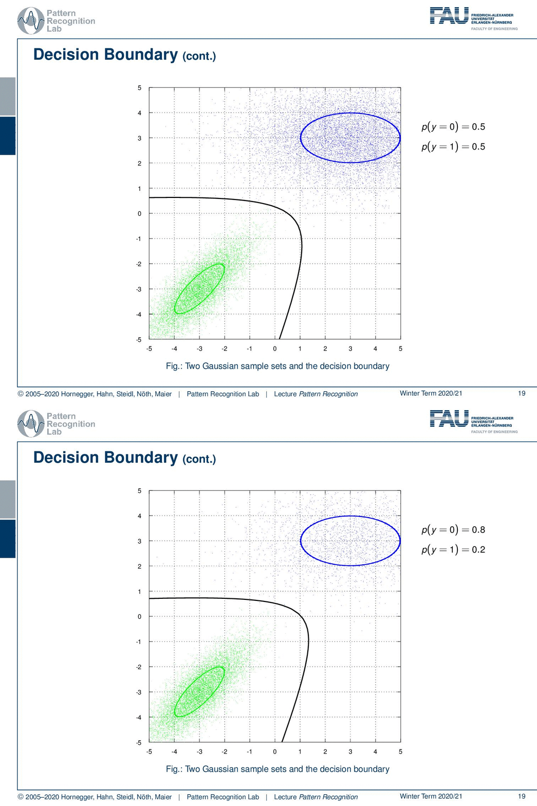
And now we can look at the decision boundary which looks like this. Now we can play a bit with the priors. If we increase the prior, then you see that our decision boundary essentially moves a bit. So this is the constant factor that we were talking about already earlier. Also, note that this is a quadratic function that is essentially intersecting with our plane of observation.
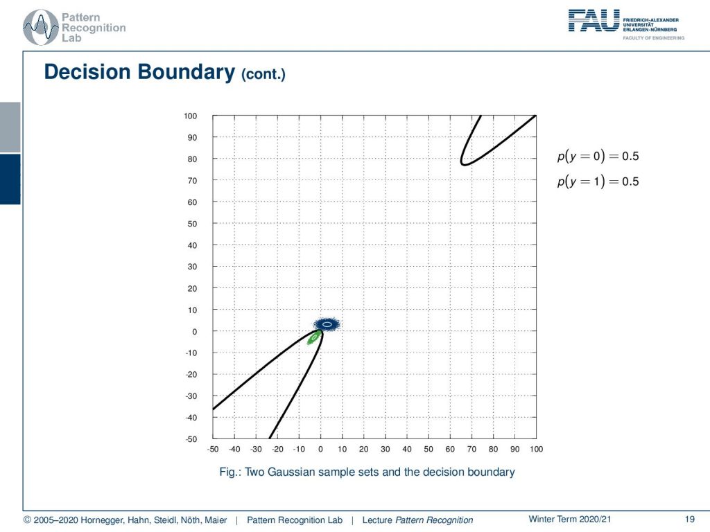
This can also imply that our quadratic function returns on the other side. So you may be quite surprised but this observation, but of course this can be explained.
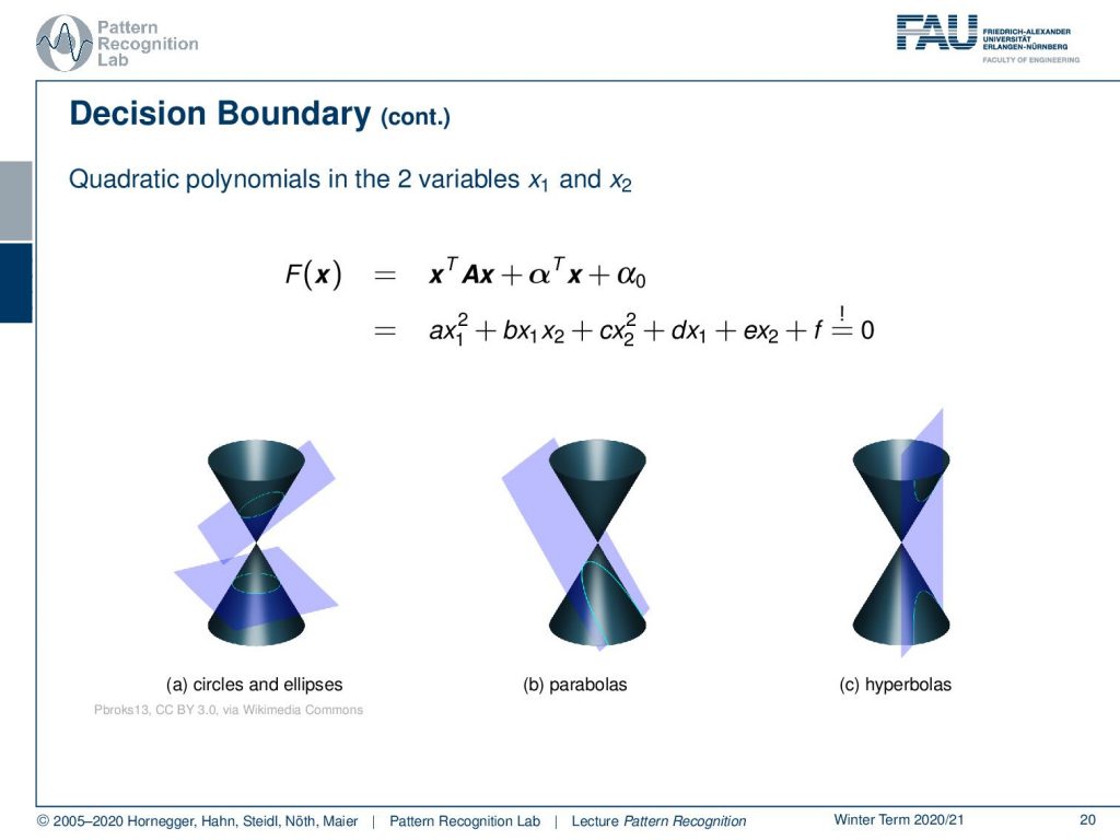
We have these quadratic polynomials in the variables x₁ and x₂. This is essentially a conic section, and we can express this either as circles or as ellipses, but it may also result in parabolas. And if you have particular configurations, you may also observe hyperbolas as we’ve seen in the previous case. This way, we can describe the decision boundary and find a closed-form solution for intersecting two different Gaussian distributions.
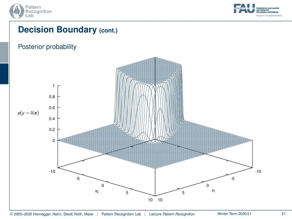
Also, note that we can also plot the posterior probabilities here. And you see that they are essentially arranged around the zero level set. So, you see that these posterior probabilities very quickly saturate in the example that we’ve seen here. So if you try to use the posterior probabilities as a kind of confidence measure for your decision, you may realize that already if you are slightly apart from your decision boundary, then you’re quite certain that you’re on the right side of the decision boundary. And of course, this is a way how we can visualize the posterior probability in a kind of surface plot for the given example.

So this brings us already to the end of this video. Next time, we want to look into cases where it’s not just Gaussian probability distributions. We also want to look into other cases and figure out whether we can use this trick with the Logistic Function there as well. I hope you liked this small video and it would be really nice to see you again in the next one! Thank you very much for watching and bye-bye.
If you liked this post, you can find more essays here, more educational material on Machine Learning here, or have a look at our Deep Learning Lecture. I would also appreciate a follow on YouTube, Twitter, Facebook, or LinkedIn in case you want to be informed about more essays, videos, and research in the future. This article is released under the Creative Commons 4.0 Attribution License and can be reprinted and modified if referenced. If you are interested in generating transcripts from video lectures try AutoBlog.
References
T. Hastie, R. Tibshirani, and J. Friedman: The Elements of Statistical Learning – Data Mining, Inference, and Prediction, 2nd edition, Springer, New York, 2009.
David W. Hosmer, Stanley Lemeshow: Applied Logistic Regression, 2nd Edition, John Wiley & Sons, Hoboken, 2000.

