
These are the lecture notes for FAU’s YouTube Lecture “Pattern Recognition“. This is a full transcript of the lecture video & matching slides. We hope, you enjoy this as much as the videos. Of course, this transcript was created with deep learning techniques largely automatically and only minor manual modifications were performed. Try it yourself! If you spot mistakes, please let us know!
Welcome back to Pattern Recognition! Today we want to review a couple of basics that are important for the remainder of this class. We will look into simple classification, supervised unsupervised learning, and also review a little bit of probability theory. So this is a kind of refresher. In case you are not that strong anymore with probability theory, you will find the examples that we have in this video very instructive.
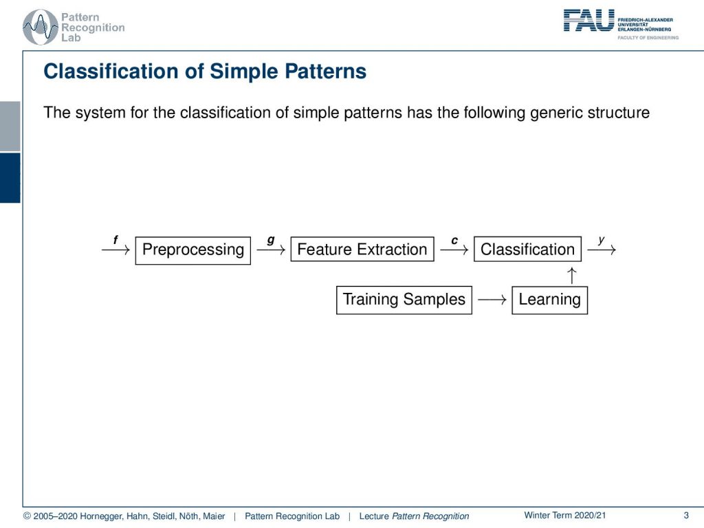
Let’s go into our Pattern Recognition basics. So, the system for classification we already reviewed in the previous videos. We have our pattern recognition system that consists of preprocessing, feature extraction, and classification. You can see that we generally use f to indicate signals that go as input into the system. Then we want to use g as a kind of pre-processed image. After the feature extraction, we have some abstract features c that are then used in the classification to predict some class y. Of course, this is all associated with training samples that we are using in order to learn the parameters of our problem.
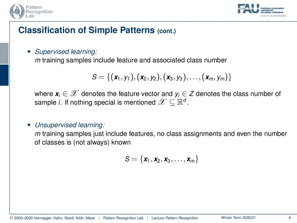
Typically, these data sets then consist of tuples. So we have some vectors xᵢ, and they are associated with some classes that are indicated here as yᵢ. These tuples can form a training data set. Now with this data set, we are then able to estimate the parameters of our desired classification system. So, this is the supervised case. Of course, there’s also the unsupervised case, in which you don’t have any classes available but you just have the mirror observations x₁, x₂, and so on. From this, you then can’t tell the class, but you know the distribution from the observed samples and you can start modeling things like clustering and so on.
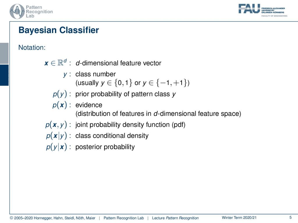
Let’s introduce a bit of notation. Generally, we will use here the vector x that is in a d-dimensional feature space. The vector is typically associated with some class number. So you could either assign it to {0, 1}. So this is a 2 class problem, but you could also indicate classes with -1 and +1. For the time being, we will look into two-class problems, but generally, we can also expand this to multi-class problems. There you can for example use class numbers, or you can also use one-hot encoded vectors. In this case, then your class is no longer a simple number or scalar, but it will be encoded as a vector. So if you attended deep learning, then you will see that we will use there this concept quite heavily. What else do we need? Well, we want to talk a bit about probabilities. So here p(y) is the prior probability of a certain class y. This is essentially associated with the structure of the problem and the frequency of that respective class. We will look into a couple of examples in the next few slides. Then we have some evidence that is generally p(x), so this is the probability of the observation x. And this is in the general case living in a d-dimensional feature space. Furthermore, there’s the joint probability. This is essentially the probability of x and y occurring together. And then there are the conditional probabilities, in particular, the class conditional probability, which is given as p of x given y. And then there is the so-called posterior probability that is p of y given x. So the posterior is essentially the probability that gives you the likelihood of a certain class, given some observation x. Now, this is fairly abstract. Let’s look into some examples of how these probabilities are constructed!
We’ll go with a very simple example that is a coin flip. In a coin flip, you can have essentially two outcomes that are heads and tails. So here, we don’t live in a d-dimensional feature space. Instead, we only have two different discrete observations that we have for our observations x. You can see here we did a coin flip. We had 18 times heads, and we had 33 times tails. In total, there are 51 observations and with these discrete observations, we can now try to estimate the probabilities. So the probability for observing heads, in this case, is approximately 35%. In the same way, I can also compute the probability for tails, which is approximately 65%. Now you see, we just have evidence but no classes. Let’s make the problem a little bit more complicated. Let’s say you are colorblind and you can’t differentiate the classes. So this is essentially the problem that we are facing. We can’t access the class, but there is some true class that is somehow hidden.
You could imagine that I actually have two different coins. So I have a red coin and a green coin. Now the red coin is producing 17 times heads and 15 times tails, while our green coin is producing heads only once and tails 18 times. So the green coin is heavily biased towards tails. Of course, we can also compute the sums of our rows which will give us these numbers. And of course, we can also compute the column sums. Here you already see that in the last row, we get essentially the same evidence as we’ve seen in the top table.
You can now look at this last row. This is essentially the case where we are color blind. We can’t differentiate the two coins and we will get exactly the same probabilities: 35% for the observation heads and 65% for the observation tails.
What else can we do? Well, we can of course also look at the last column. And here you can see essentially our class priors. The probability of using the red coin is approximately 63%, and the probability of using the green coin is 37%. So you could argue if somebody is using those two coins, then he’s trying to use this kind of biased coin. Not in all of the instances, but the person is mixing this coin in on occasions because probably you don’t want to be caught cheating. So you just mix it in let’s say 37 of the cases because of course, you also want to win quite frequently. And in the other cases, you don’t want to get caught, so this is why you’re using the other coin. Makes perfect sense right? So let’s look a bit into the joint probabilities.
Now, this would be the probability that you observe heads and the red coin at the same time. Here you can see this is 17 times with 51 observations in total. So this is equal to about 33% likelihood. Of course, we can do similar things with tails and the green coin, which would equate to approximately 35 percent. Now, if we want to compute those numbers we need access to the class distribution. So we need to know which coin is available, and we also need to know what the actual observation, what our evidence was. Now, what else can we do with this nice table?
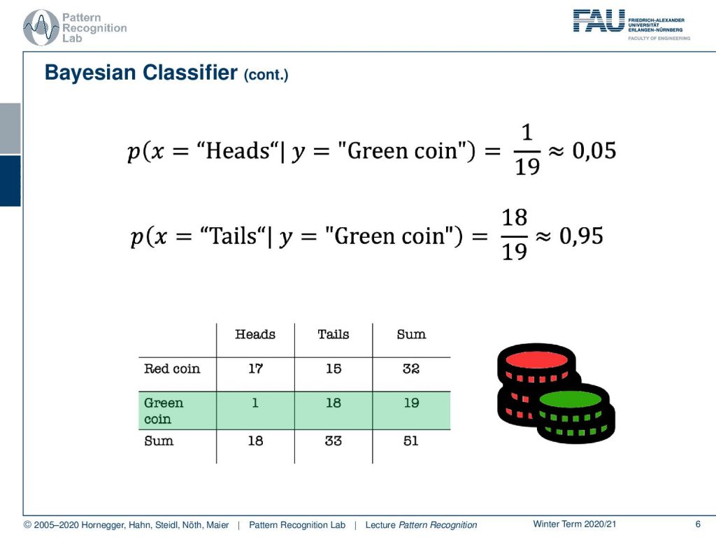
We can of course analyze our coin. Here you see that our green coin is the one that is biased towards tails, and you can compute the probability for heads given the green coin. So if I start tossing this, I will only have a 5% chance of producing heads, and I will have a 95% chance of producing tails. Now, this is essentially the information that I don’t have. I get some information, I get the observation heads and tails because I’m colorblind.
And now I’m interested in figuring out whether it’s the red coin or the green coin. Now, if I observe tails, then I know that I have observed tails, so I can already fix that. And then I compute the probability for the red coin, so this is one of the two classes. The other class is the green coin, and you see that the probabilities are 45% and 55%. So if you observe tails, then this is not very strong evidence of which coin was actually tossed. Let’s look into the other case.
So let’s say we observe heads. Now, if you observe heads, the probability for the red coin is approximately 94% and the probability for the green coin is only 6%. Because in most of the cases where heads is produced, of course, the red coin was used. So observing heads, in this case, is very strong evidence, that the red coin was used. And you can already see this is a very typical Pattern Classification problem. So we want to derive the class information about the coin from the observed evidence. And you already see that it’s hard. But if you have distributions like this one, then you can get very interesting and very good evidence from our experiments. Let’s formalize this a little bit.
We’ve seen that the joint probability density function here with x and y can be decomposed into the prior. So the probability of using a certain coin times the class conditional probability density function. Obviously, the same joint pdf can be produced by using the probability of the evidence times the posterior probability. So you can see we can express the same joint probability density function using those two decompositions.
Now, if I know this identity, then I can very easily construct the so-called Bayes Theorem. The Bayes Theorem tells us that the probability for a class y, given the evidence x, can be expressed as the prior probability of the class y times the probability of x given y. This is divided by the probability of x. Now, the probability of x generally can also be expressed as a marginalization over the entire joint probability. And now you see that observing this joint probability density function is pretty hard. But we can use our trick of decomposition again. So we can see that this can be decomposed into the prior of all the classes, and this is multiplied with the probability of observing our x given the respective class. This is called marginalization. The nice thing here is that our y is always discrete. So we have a discrete number of classes, which allows us to express this as a sum.
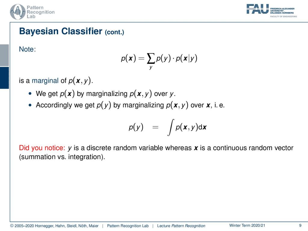
This is the marginal of the joint probability density function. And we can essentially get that by marginal analyzing over our classes y. If we want to do something similar for the prior probability of class y, then we would have to marginalize over x. And if you want to do that, then you can already see that we would have to have a continuous integral over the entire domain of x. Simply because in our case, or in most cases that we will look at in this class, x is not discrete as in the previous example but instead it is a continuous vector space. So we have to compute the integral over this entire vector space. This is already the end of our small introduction to the different probability theory.

In the next video, we want to talk about the Bayesian Classifier and how the Bayesian Classifier is related to the optimal classifier. I hope you liked this little video and I’m looking forward to seeing you in the next one! Thank you very much for watching and bye-bye.
If you liked this post, you can find more essays here, more educational material on Machine Learning here, or have a look at our Deep Learning Lecture. I would also appreciate a follow on YouTube, Twitter, Facebook, or LinkedIn in case you want to be informed about more essays, videos, and research in the future. This article is released under the Creative Commons 4.0 Attribution License and can be reprinted and modified if referenced. If you are interested in generating transcripts from video lectures try AutoBlog.
References
Heinrich Niemann: Pattern Analysis, Springer Series in Information Sciences 4, Springer, Berlin, 1982.
Heinrich Niemann: Klassifikation von Mustern, Springer Verlag, Berlin, 1983.
Richard O. Duda, Peter E. Hart, David G. Stork: Pattern Classification, 2nd edition, John Wiley & Sons, New York, 2000.