
These are the lecture notes for FAU’s YouTube Lecture “Pattern Recognition“. This is a full transcript of the lecture video & matching slides. We hope, you enjoy this as much as the videos. Of course, this transcript was created with deep learning techniques largely automatically and only minor manual modifications were performed. Try it yourself! If you spot mistakes, please let us know!
Welcome back to pattern recognition. Today we want to continue our short introduction to the topic and we will talk about the postulates for pattern recognition and also some measures of evaluating the performance of a classification system. So, looking forward to showing you some exciting introduction to the topic.
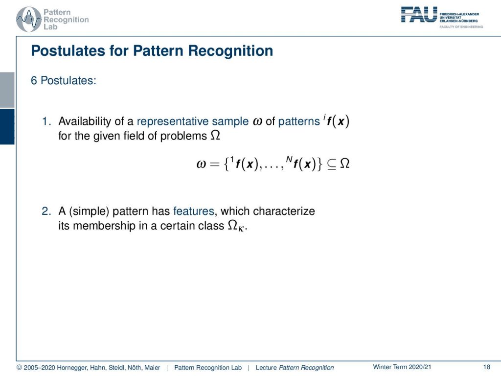
For classical pattern recognition we have six postulates and these six postulates, essentially tell us on which occasions it’s a good idea to apply a pattern recognition system. The first thing that you should keep in mind is that you should have available a set of representative patterns and these are about our problem domain Ω and the patterns f(x) are essentially the instances of the observations that we want to use to decide for the class of the respective pattern.
Next, a simple pattern should be constructed from features that characterize its membership and the membership is then assigned to a certain class Ωк. So, this is crucial you have to have observations with characteristic features otherwise you will not be able to assign them to a class. This brings us already to the third postulate there should be a kind of compact domain in this feature space that labels or brings together the same class and typically those areas should have a small intraclass distance meaning that the distance between observations of the same class should be small and observations between samples of different classes.
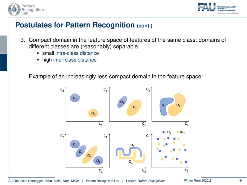
So, the inter-class distance should be high as you can see above. Here we have a couple of examples for the distribution in the feature space and you see on the top left this is a pretty clear case. Also, the center top image is still a separable case they maybe not trivial but in the top right case you can still separate the two classes, of course no longer with a line but with something non-linear. Then of course also the classes could be intermixed so here you see different distributions of classes and you see that we are still able to separate the two when we figure out where the instances of a certain observation are located. Also, there could be more complex structures in the high-dimensional feature space as shown in the bottom center. The thing that you want to avoid is the configuration on the bottom right. Here it’s very hard to separate the two because it looks like the samples were essentially drawn from the same distribution. If you have observations like this then you may want to think about whether your feature space is a very good one and maybe you want to extract different features or, even it might be the case that the problem is not solvable.
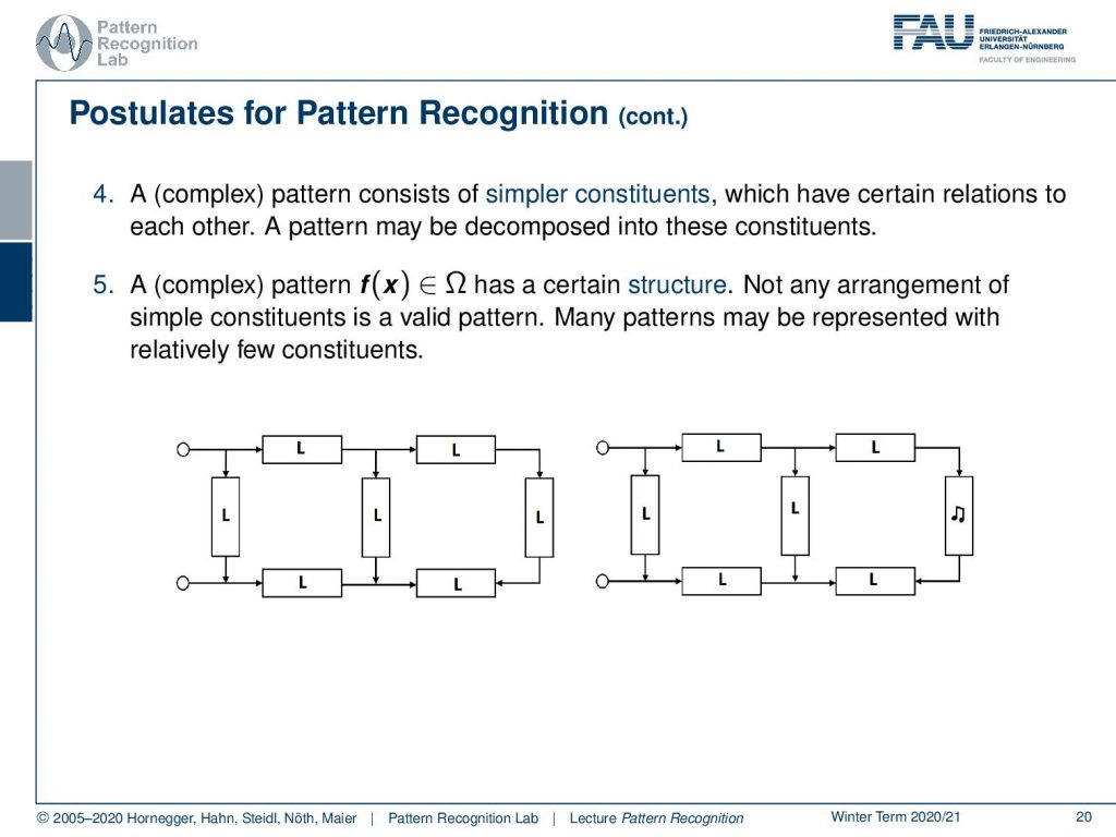
So, this can of course also be the case that there might be classes that you can’t separate with the observations that have been given a fourth postulate is that typically a complex pattern should consist of simpler parts and this then should be also expressible in relation to each other so a pattern should be decomposable into those parts.
Then also a complex pattern should have a certain structure, not any arrangement of simple parts should construct a valid pattern and this means that many patterns can be represented with relatively few constituents. So here you see an example on the left-hand side this is a valid pattern. On the right-hand side, you see parts of the image are not valid as you can see with the musical note on the transistor on the right. So this is not a valid pattern and therefore we might want to consider also the case to reject patterns and the last postulate is that two patterns are similar if their features or, simpler constituents differ only slightly.
Okay, if we find that these postulates are applicable to our problem, then we can apply the methods of pattern recognition. So once you apply the pattern recognition then you probably also want to measure whether your classification is successful and therefore we typically use measures of performance and one way of displaying how well your system is performing is looking at the so-called confusion matrix.
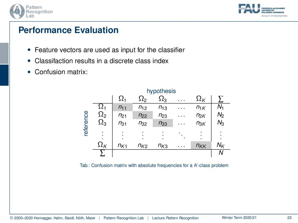
So, in this confusion matrix, we have essentially one column for every class and one row for every class and you see above that we have on the columns the hypothesis and on the rows the references. So, you essentially end up with a square matrix where K is the number of classes and this then allows us to determine how many confusions have been taken place and it will also tell you which classes are more likely to be confused with which other class. So, this is a very nice means of displaying the classification result and it will work for several classes. Obviously, this might not be the right choice if you have thousands of classes but for let’s say 10 to 20 classes; this is still a very good means of actually displaying the classification result.
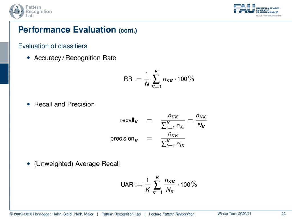
If you want to break it down into fewer numbers, one thing that you can do is you can compute the accuracy or, recognition rate and here you simply take the sum over all correct classifications and you divide by the total number of observations and this gives you the recognition rate. The recognition rate may be biased towards a certain class and therefore, also other measures have been introduced. So here we have the recall and precision where you essentially see that the recall measures the number of correct classifications for that specific class over the total number of observations for this class and the precision then is the associated measure. Again you look into the correct classifications for the class, but then you essentially take the transposed row for normalization. So you normalize with all detected observations of that class then there are also measures like the average recall and here you have essentially the recall or class wise recognition rate. You essentially then compute the sum over all of the class-wise recognition rates and compute the average over that and this means that you essentially weigh every class as equally important in contrast to the recognition rate where you weigh everything with the relative frequency as the classes occur. So this is a measure that will help you to figure out whether you have some bias towards a certain class and it will be ideally high if you have a similar recognition rate for all the classes.
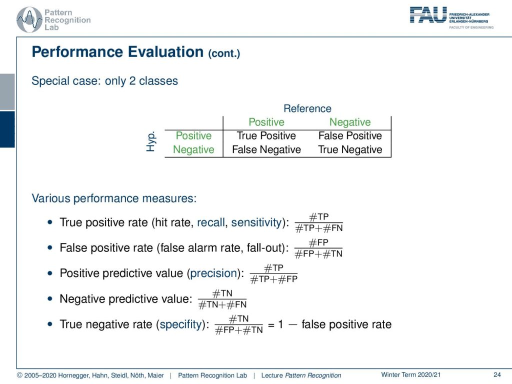
Then if you only have two classes you can also do more elaborate measures of classification measurement. So here you essentially end up with the true positive rate, the false positive rate, the positive predictive value which is essentially the precision, the negative predictive value, and the true negative rate which is the specificity. So, this can be expressed as (1 – the false positive rate).
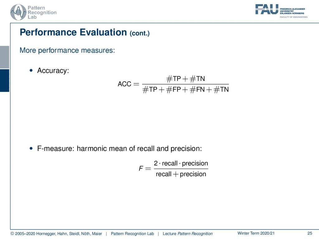
This then brings us to the accuracy and the accuracy is given as the true positives plus the true negatives divided over the total number of observations and you can also construct the F-measure which is the harmonic mean of recall and precision and you can formulate it as 2 times recall times precision over recall plus precision.
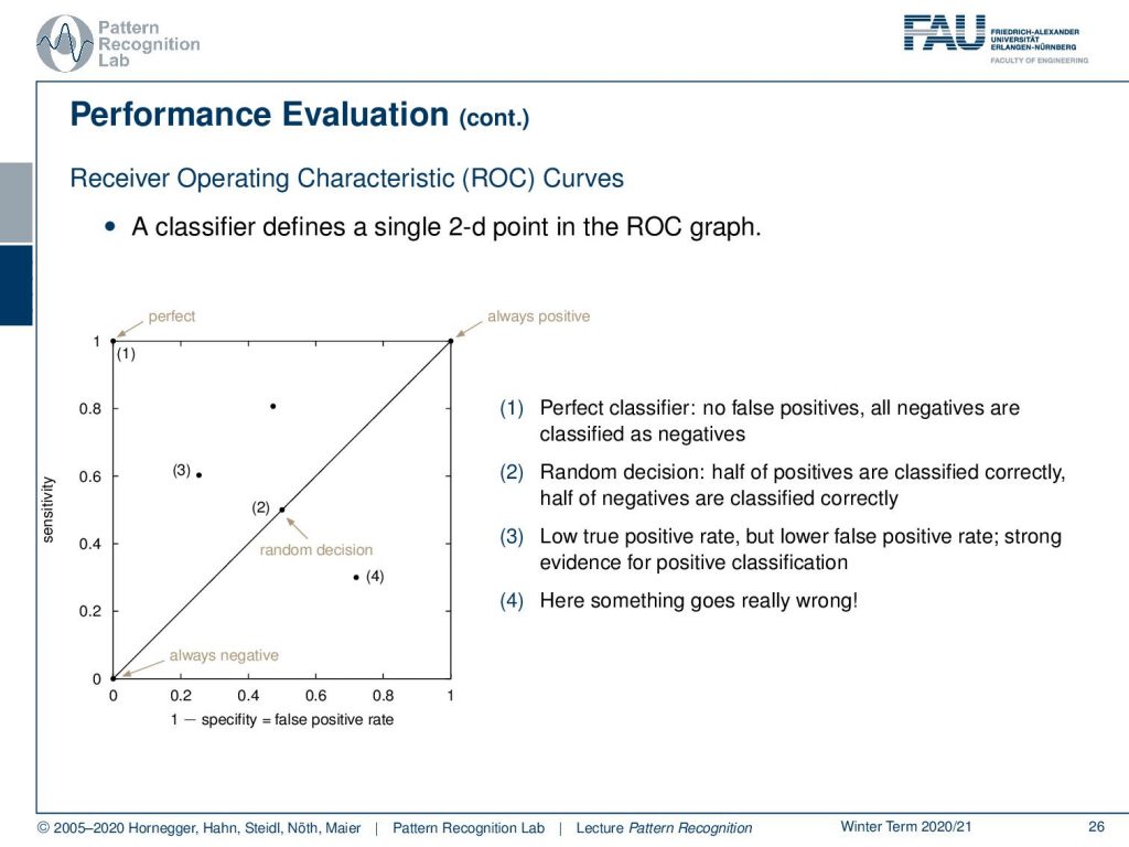
One very sophisticated way of looking at different classifiers is the so-called receiver operating characteristic curve, the ROC curve, and this can essentially look at the classification with different thresholds so here you essentially define this over a 2D space in the ROC graph and you have the sensitivity and one minus the specificity that you can actually display here and this can then be essentially determined as the ROC curve by varying different thresholds. You see that the line that is indicated through zero-zero and one-one is the random classification line so a random classifier will exactly follow this line and typically you want to be in close proximity of the perfect classifier, that would have essentially a one on the sensitivity axis and a zero on the one minus specificity axis. So, this would then be the perfect classifier. A random decision again is on the line that is separating this space and of course, you want to avoid any kind of classification that is below the line of random classification that is indicated before here. so this is really wrong. So, there you must really have a mistake in the classification system. Essentially in these two-class problems, you would just have to flip the decision of your classifier and you would be on the other side of the line. So this is probably a bug in the evaluation. If you have outcomes below random classification you really should check something is going wrong.
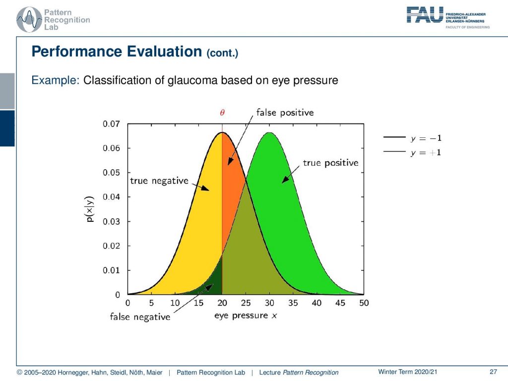
Let’s have a look into the performance evaluation in more detail so what you typically have is a distribution over the true positives and the true negatives and then the problem is often that you can’t separate the two ideally and depend on your threshold θ. Here you will introduce a different number of false positives and if you adjust now this threshold you will see that you can then determine a different number of true negatives and true positives. So, you essentially change the classification result determined by this threshold.
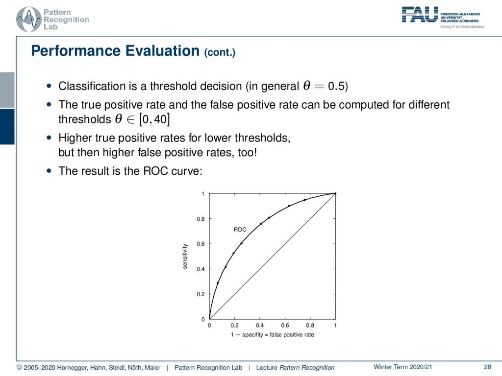
So, if you know vary this threshold you can see that this will give us a curve and this should be a curve as in the shape here as shown in the bottom of the slide so if you classify of course all to the one side then you end up at zero-zero and if you classify everything to the other side you end up at one-one so these two points are always part of the ROC curve and then you can vary your threshold along this curve and the closer the curve runs to the top left of the image the better is your classifier.
This then often gives rise to other measures that are for example called the area under the curve and you want this measure to be close to one because if it were one then you would essentially have constructed the perfect classifier.
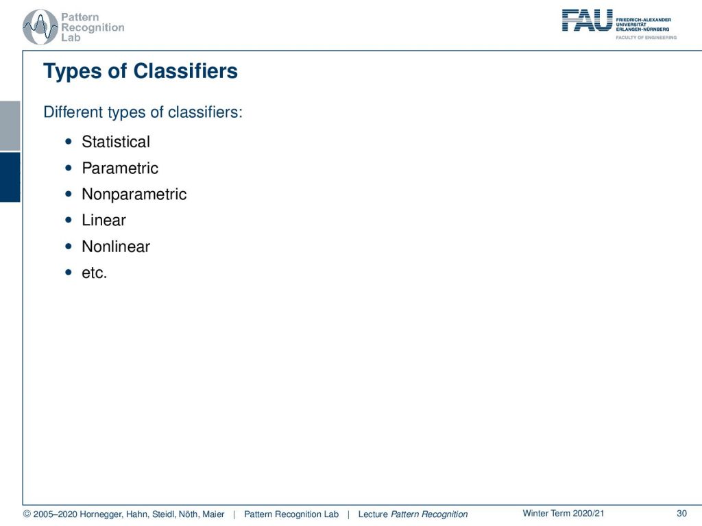
So, there are many different kinds of classifiers this starts with statistical classifiers there are parametric classifiers non-parametric classifiers linear and non-linear ones and essentially we will talk about many different choices of classifiers throughout this lecture.
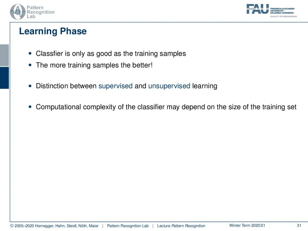
All of them share a learning phase and in this learning phase, the parameters of the respective classifier are determined from some sample observations, and typically the more training samples they have the better the classification result is. There is, of course, the distinction between supervised and unsupervised learning. In the supervised case, you have observations x and class labels y and in the unsupervised case you only have observations x and you try to figure out some kind of learning procedure which then typically also goes into the direction of clustering. There are certain choices of classifiers where the computational complexity actually depends on the size of the training data set. This is, for example, the before mentioned nearest neighbor and k nearest neighbor classifiers where you essentially have to browse through the entire training set. So, this brings us already to the end of this lecture.

In the next lecture, we want to look into the first ideas of classification we will look into the base theorem and then talk about the base classifier of course.
I also have some literature for you. I really recommend the book by Duda and Hart. This is pattern classification, a very nice book. Then of course The Elements of Statistical Learning by Hastie and the book by Bishop Pattern Recognition and Machine Learning.
Also, if you want to have some further reading on this particular video then I recommend Duda and Hart and of course the book by Niemann “Klassifikation von Mustern” which is available in the second edition under this link, unfortunately, it’s only available in german.
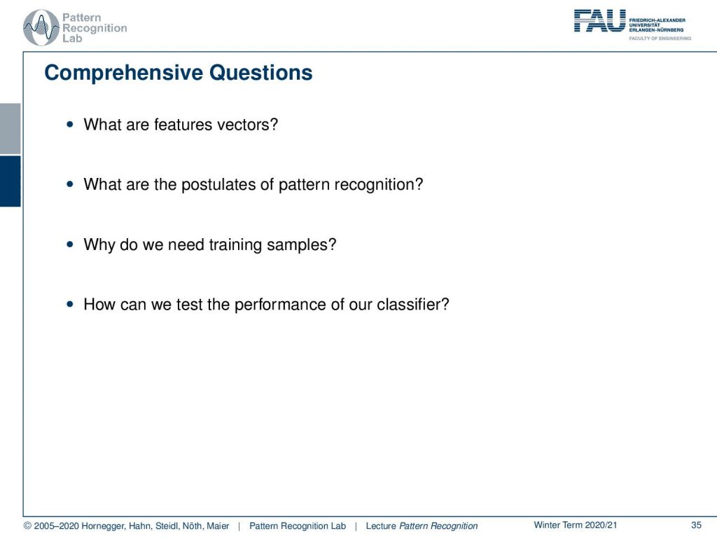
I have some comprehensive questions for you that may help you with the exam preparation. So, for example, what are feature vectors? What is feature extraction? What are the postulates of pattern recognition? Why do we need training samples at all and how can we test the performance of our classifier?
Thank you very much for listening and looking forward to seeing you in the next video!
If you liked this post, you can find more essays here, more educational material on Machine Learning here, or have a look at our Deep Learning Lecture. I would also appreciate a follow on YouTube, Twitter, Facebook, or LinkedIn in case you want to be informed about more essays, videos, and research in the future. This article is released under the Creative Commons 4.0 Attribution License and can be reprinted and modified if referenced. If you are interested in generating transcripts from video lectures try AutoBlog
References
1. Richard O. Duda, Peter E. Hart, David G. Stock: Pattern Classification, 2nd edition, John Wiley & Sons, New York, 2001
2. Trevor Hastie, Robert Tibshirani, Jerome Friedman: The Elements of Statistical Learning – Data Mining, Inference, and Prediction, 2nd edition, Springer, New York, 2009
3. Christopher M. Bishop: Pattern Recognition and Machine Learning, Springer, New York, 2006
4. H. Niemann: Klassifikation von Mustern, 2. überarbeitete Auflage, 2003