These are the lecture notes for FAU’s YouTube Lecture “Pattern Recognition“. This is a full transcript of the lecture video & matching slides. We hope, you enjoy this as much as the videos. Of course, this transcript was created with deep learning techniques largely automatically and only minor manual modifications were performed. Try it yourself! If you spot mistakes, please let us know!
Welcome back to pattern recognition! Today we want to talk a bit about norms and we will look into different variants of vector norms, matrix norms, and have a couple of examples of how they are actually applied.
Let’s look into norms and later on also norm dependent linear regression. So, we’ve seen that norms and similarity measures play an important role in machine learning and pattern recognition. In this chapter, we want to summarize important definitions and facts, and norms. I think this is also a very good refresher if you’re not so familiar with norms. This video will be a very good summary of the most important facts on norms. So, we’ll consider the problem of linear regression. Then later in the next video for different norms. But in this video, we’ll mainly talk about norms and their properties. Later we also look briefly into the associated optimization problems.
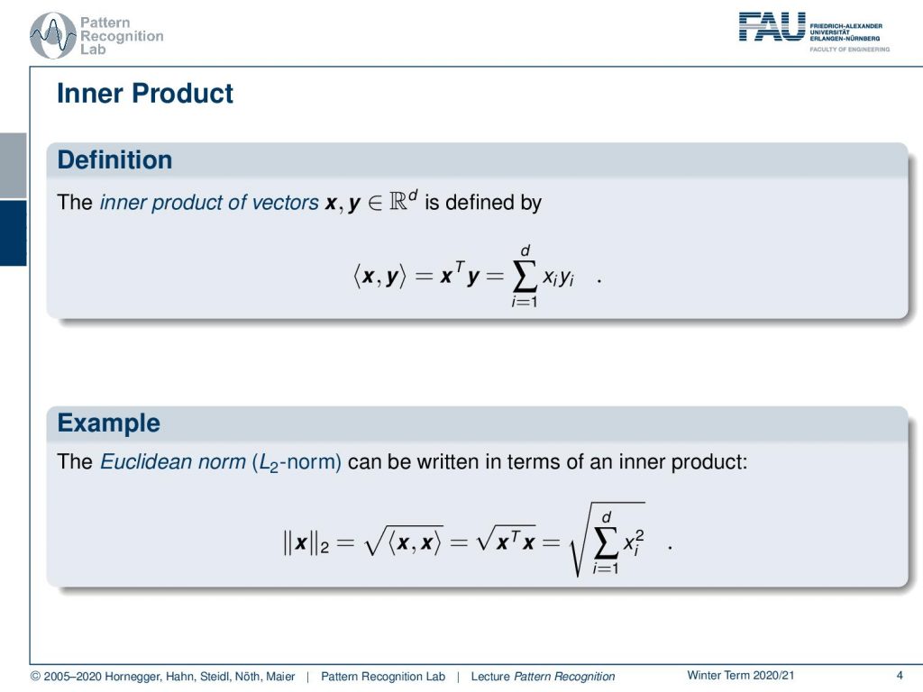
Let’s start with the inner product, the inner product of two vectors that we already used in this lecture. We write this up as x transpose y and this essentially is the sum over the element-wise multiplication. This can then be used to define the euclidean L2 norm. So this is essentially the inner product of the vector with itself and then we take the square root. So we can write this as x transpose x square root or, you could say that element-wise is the square summed up and then taken the square root.
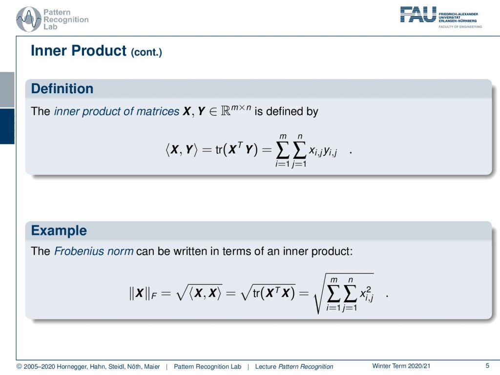
Also, we can define inner products of matrices and if we want to do that then we see that the inner product of a matrix is essentially x transpose y. Then we take the trace of the resulting matrix. This then results in a sum over all the elements of x multiplied with all the elements of y. Then we compute the essentially two-dimensional sum here because they’re matrices. But we mix all the elements with each other and sum them up. Now if you follow this definition then you can find the Frobenius norm as the inner product of x with itself. So this means that we essentially square all of the elements and then sum them up. So this is the Frobenius norm.
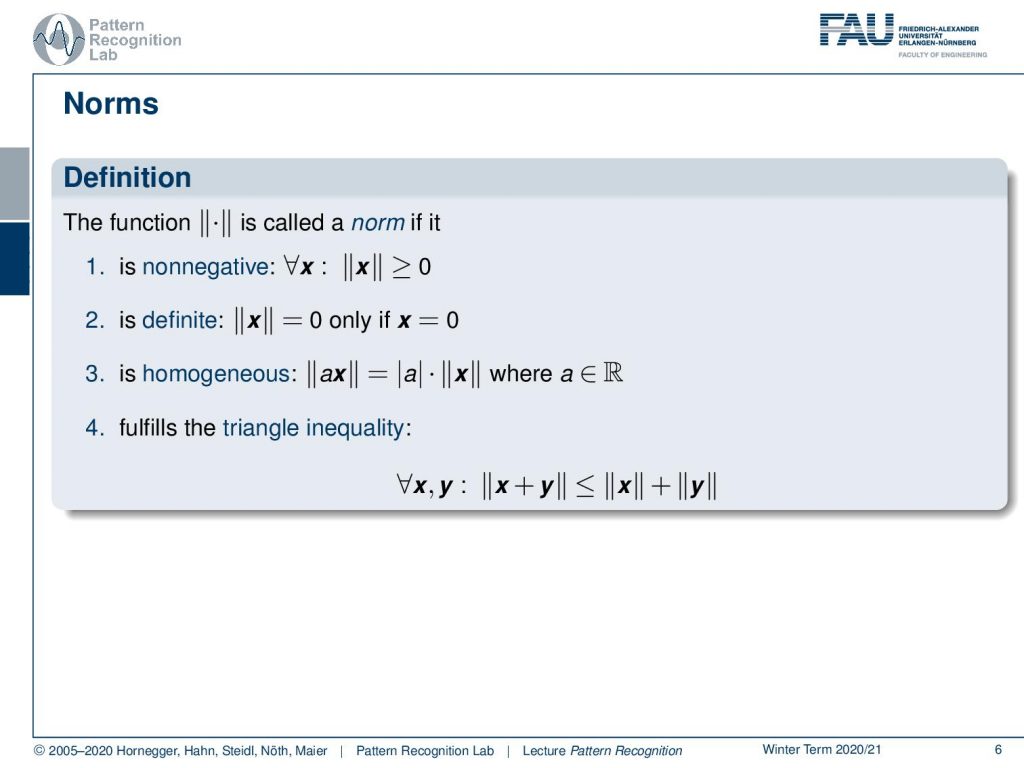
What else do we have? What’s a norm actually the function that we indicate with these double bars is called a norm. If it is non-negative. So, the result of the norm is always 0 or greater than 0 for all given x. Then it should be definite, which means that it will be 0 only if all of the entries of x are 0. It should be homogeneous which means that if you multiply a with x and a is a scalar value and you take the norm then this is the same as taking the absolute value of a and multiplying it with the norm of x. This is of course true for scalar values. Then it should also fulfill the triangle inequality which means that for all x and y. If you have some x and you add y and take the norm then this should be lesser or equal to the norm of x plus the norm of y, also known as the triangle inequality.
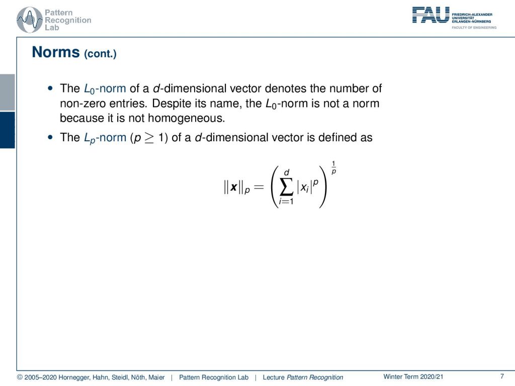
Then we can also find other norms for example the L0 norm which is essentially denoting the number of non-zero entries. Despite its name, it’s not really a norm. So we will see that and you see that often used also in Richard, the l0 norm and also other variants that are actually not norms. But they’re used in this context. So generally this will allow us to define an Lp norm and now p is a scalar value. Note that this is small caps p and it’s defined as a norm with p greater or equal to one of a d-dimensional vector. Then you can compute this essentially with the element-wise xi to the absolute value to the power of p then summed up. Then you take the p-root of the respective sum. Technically you can also do this with values lower than one but then you end up with constellations that no longer fulfill all of the previous norm properties. In literature, you can also find this as a zero norm or as an L0.5 norm, and so on. So, you essentially use this same idea of computing them but you use values that are smaller than one for this.
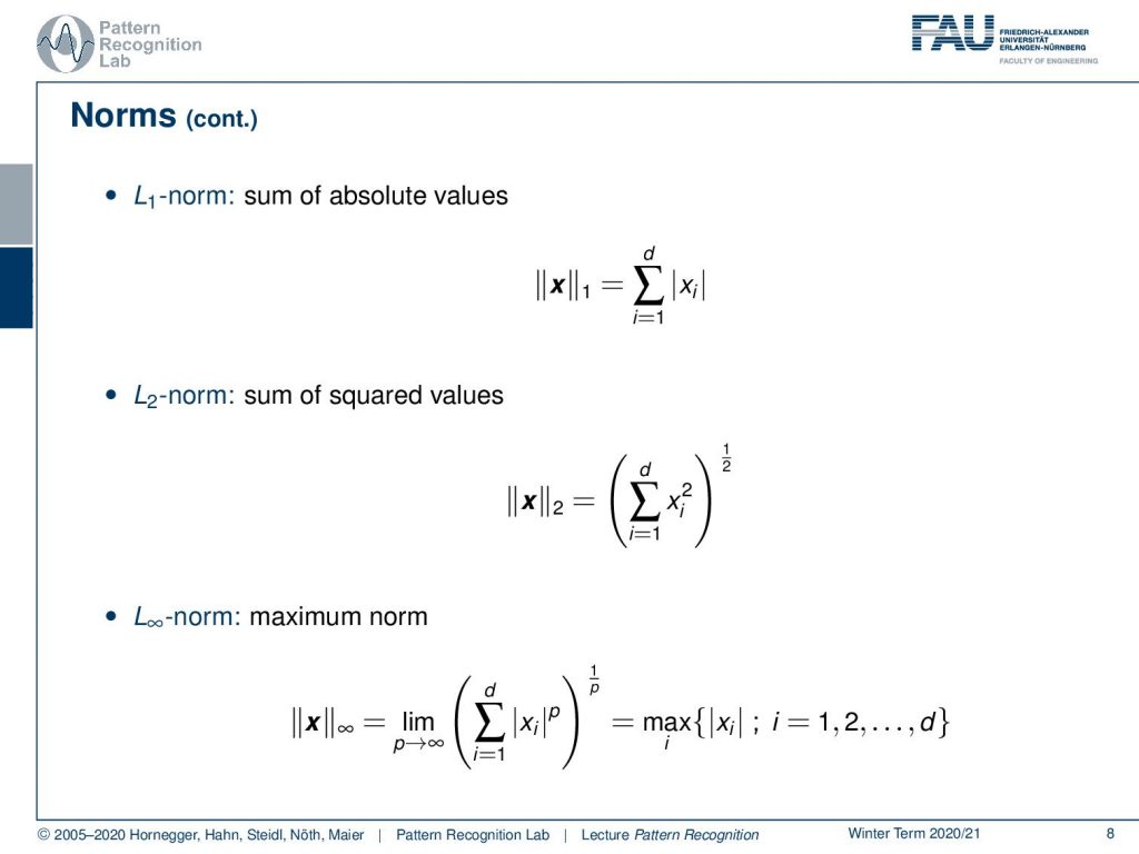
Now let’s look into real norms so there’s the L1 norm, which is essentially the sum of absolute values. Then there’s the L2 norm that is essentially the sum of squares and the square root. Then there are also other norms following this direction up to the L infinity norm and this is also called the maximum norm. Here you essentially pick the maximum absolute value that occurs in the vector and returns it as the respective result of the norm.
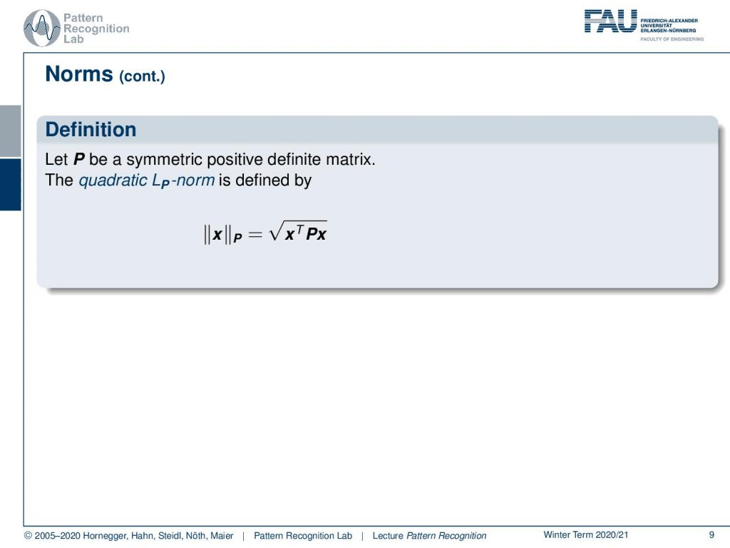
So, there is also Lp norm but now P is a capital P and bold. This is a matrix and if it is a symmetric positive definite matrix then the quadratic Lp norm can be given in the following way. So, this is essentially x transpose times P times x. It’s essentially a weighted distance to itself weighted by P. Then you take the square root.
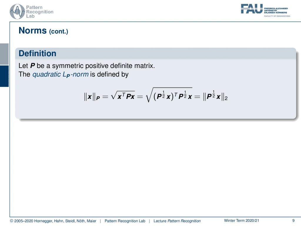
So you can also write this up in the following way: if you split P but you need to be able to decompose P and if you use a symmetric positive definite matrix it will be possible to do this factorization. Then you can also use this definition and this way you could also rewrite it to P to the power of 0.5 so this decomposition times x and then the L2 norm.
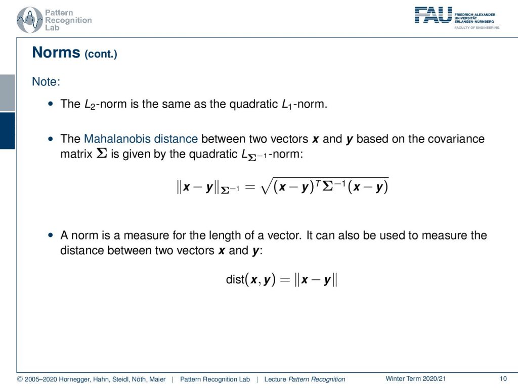
The L2 norm is the same as the quadratic one norm. You can also write up the Mahalanobis distance between two vectors using the inverse of the covariance matrix. So, this would then be the quadratic Lsigma inverse norm and here you see that it is essentially a kind of Lp norm with the inverse covariance matrix as the respective scaling norm for the distance. We can see that generally, a norm is a measure for the length of a vector. It can be used to measure the distance between two vectors x and y. So, depending on the kind of norm that you’re taking, you’re taking a particular interpretation of the distance between the two vectors.
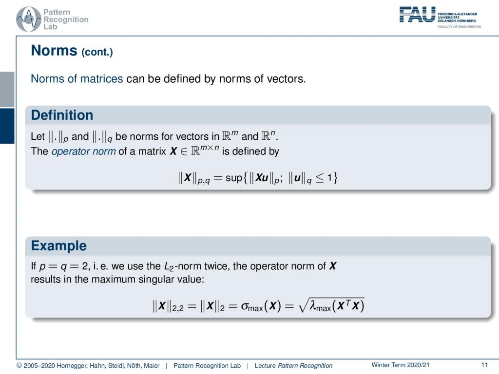
You can also define norms for matrices and there you use essentially norms of vectors. So, if you have two vector norms let’s say the p and the q norm for vectors in our m and our n. Then you can define the operator norm of a matrix X that is living in an m times n space. Then you can find this as the supremum of X times u and p norm of that and the q norm of u limited by 1. so let’s look into some example. If we have p and q equals to 2 this means that we use the two norm twice and the operator norm of X results then in the maximum singular value. So, the matrix norm of ||X||2,2 equals to the matrix norm of ||X||2 and this is given as the maximum singular value of x. This can also be computed as the maximum eigenvalue of X, transpose X and then you take the square root so this would be equivalent.

Also, an important concept with respect to norms also for visualization is unit balls. The unit ball is the set of all points that fulfill the property that the norm is lower to one. This then gives rise to the unit ball of that respective norm.
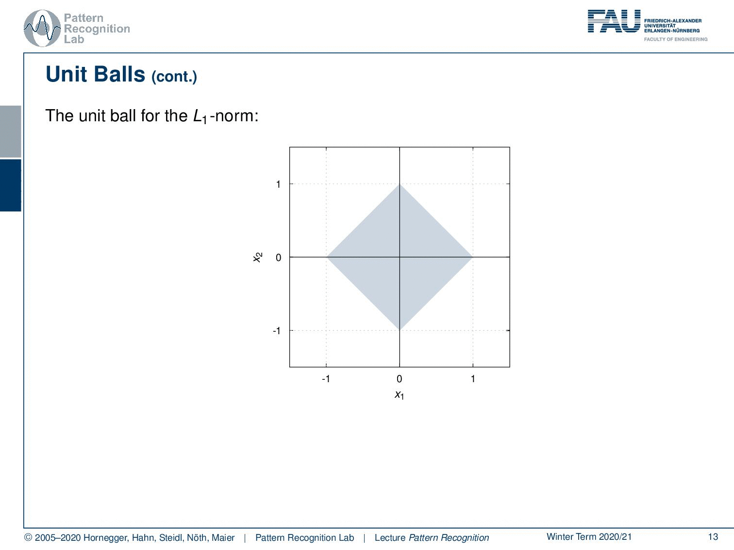
We can very quickly see the unit ball for example for the L1 norm isn’t actually a ball. But it looks more like a diamond. We can then go ahead and look into the two norms, there we have much more the impression of a ball because it’s round. So, this is the typical impression of the L2 norm unit ball. For the maximum norm, you see that this essentially becomes a square where we have all the elements that are essentially between -1 and 1 on both axes of the coordinate system. A p norm generally would have the following form so you know that if you apply a matrix that’s essentially a rotation and scaling on the major and minor axis of the resulting ellipse. So the unit boyfriend Lp norm generally takes this form of ellipses.
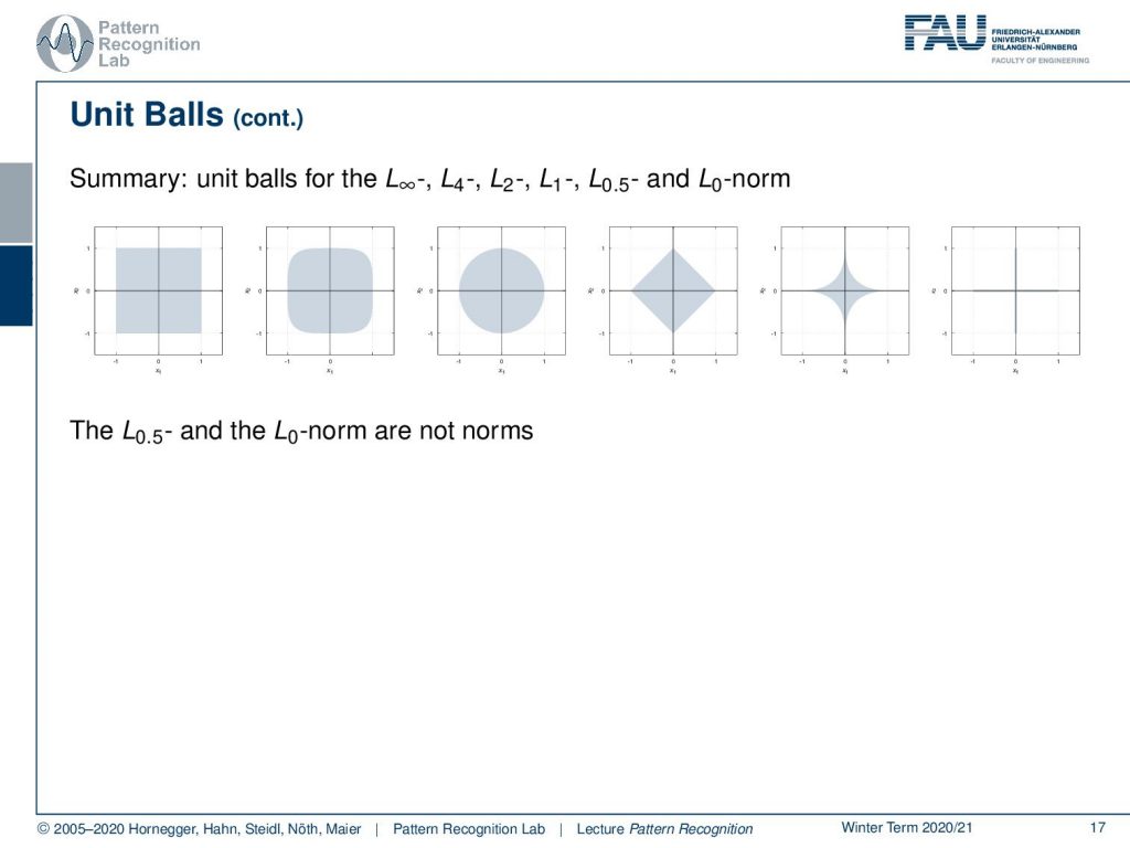
We can also have a look at the unit balls for other norms. If we start with the maximum norm, the four norm, the two norm, the one norm, and then you see that we can also go-ahead to the not really norms but also numbers that we can compute and use an optimization the 0.5 norm and the L0 norm. They are then no longer convex optimization problems, but you can generally also use them if you want to perform optimization. Yet the resulting optimization problem is typically pretty hard.

Okay, so this is our short introduction to norms and I hope you found this quite interesting. In the following couple of videos, we will put these norms into use and the first thing that we want to look at is using these norms for regularizing regression problems. So, I hope you enjoyed this little video and I’m looking forward to seeing you in the next one. Bye Bye!
If you liked this post, you can find more essays here, more educational material on Machine Learning here, or have a look at our Deep Learning Lecture. I would also appreciate a follow on YouTube, Twitter, Facebook, or LinkedIn in case you want to be informed about more essays, videos, and research in the future. This article is released under the Creative Commons 4.0 Attribution License and can be reprinted and modified if referenced. If you are interested in generating transcripts from video lectures try AutoBlog
References
- G. Golub, C. F. Van Loan: Matrix Computations, 3rd Edition, The Johns Hopkins University Press, Baltimore, 1996.
- Lloyd N. Trefethen, David Bau III: Numerical Linear Algebra, SIAM, Philadelphia, 1997.
- S. Boyd, L. Vandenberghe: Convex Optimization, Cambridge University Press, 2004. ☞http://www.stanford.edu/~boyd/cvxbook/
- Compressed sensing is one of the most recent hot topics in pattern recognition and image processing. An excellent source is: http://www.dsp.ece.rice.edu/cs
- A recent workshop on compressed sensing at Duke University: http: //people.ee.duke.edu/%7Elcarin/compressive-sensing-workshop.html.