
These are the lecture notes for FAU’s YouTube Lecture “Pattern Recognition“. This is a full transcript of the lecture video & matching slides. We hope, you enjoy this as much as the videos. Of course, this transcript was created with deep learning techniques largely automatically and only minor manual modifications were performed. Try it yourself! If you spot mistakes, please let us know!
Welcome back to Pattern Recognition. You’ve seen that we discussed the Linear Discriminant Analysis and also associated classification. Today, we want to look into a couple of applications of this technique. And we want to show you that this is not just something that you find in textbooks, but this is actually being used in several different variants.
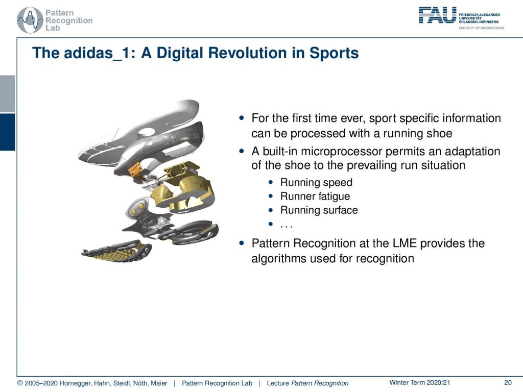
Here you see the adidas_1, which is a digital revolution in sports. This is actually work that has been done by a colleague of mine, Björn Eskofier. They significantly contributed to the development of this intelligent shoe. So this was the first time ever a shoe had embedded sensing. The sole of the shoe was constructed in a way that it had a sensing and a motor element. So the shoe could adjust the stiffness of the sole. This is very interesting, because if you are running cross-country, then sometimes you’re on hard soil. In these cases you want your shoes all to be very soft. But in other cases, you’re running on very soft soil, and in these cases, a hard shoe sole can actually prevent injury. So an intelligent shoe that would then adjust to the floor, to the soil, to the terrain that you’re running on is a very good idea to prevent any kinds of injury during sports. This shoe was made into a product by Adidas. So you could actually buy it in the stores, and the sensing and recognition system has been developed at our lab.
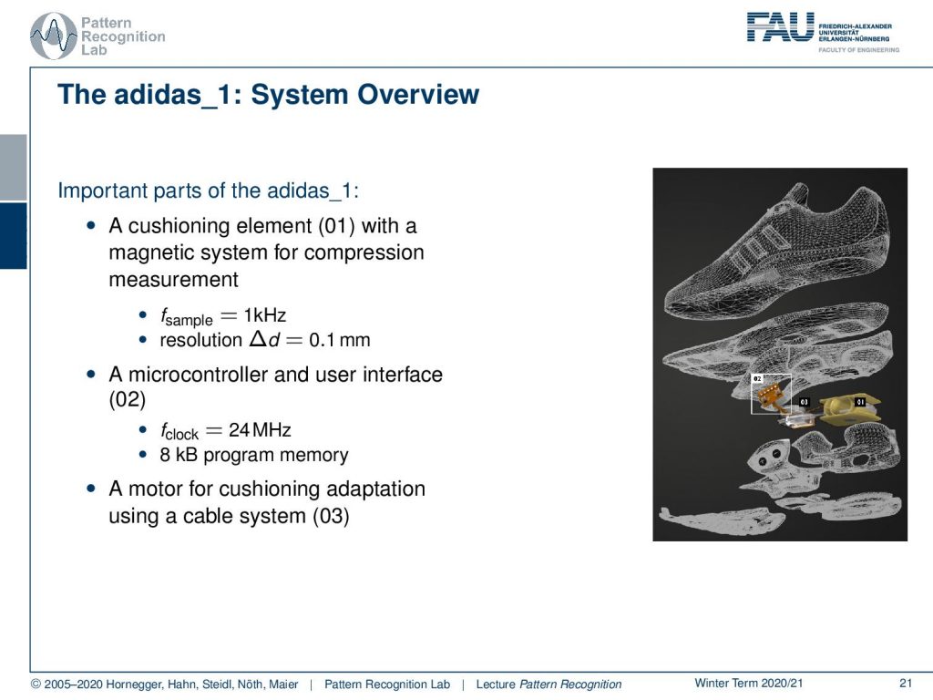
So, what is the overview? Well, you had this cushioning element that is indicated by 01 here, which has a magnetic system for compression measurement. Then you had a microcontroller and a user interface that are essentially buttons on the shoe. This had a clock frequency of 24 MHz, and you only had eight kB of program memory. Then, there was a motor for adapting the cushion using a cable system. You see, the challenge here is that you can compute only very little in a shoe. So this embedded system really needs fast processing and simple methods in order to perform the classification. This is exactly where our ideas with feature transforms now come in.
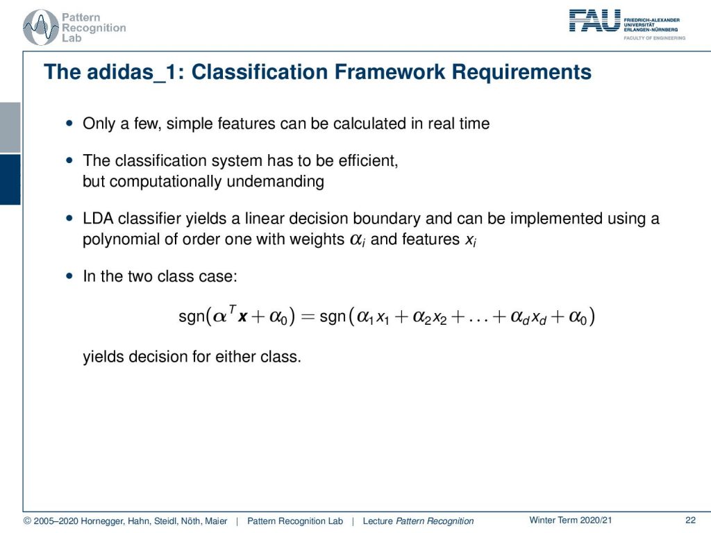
You can only do a couple of very simple features on the shoe, and they have to be calculated in real-time. Then the classification itself also has to be very efficient because you have strong memory and compute limitations. Therefore, the LDA classifier can really help us here. The nice thing with the LDA classifier is that it essentially maps this two-class problem into a linear decision boundary. Therefore, we can approximate this two-class problem now with a polynomial of order one. We simply have to introduce weights αi and features xi in order to compute that. So the actual decision then is performed as the sign of the projection onto this class boundary with the respective bias. And then you decide whether you’re on the one side of the plane or the other side of this high dimensional hyperplane.
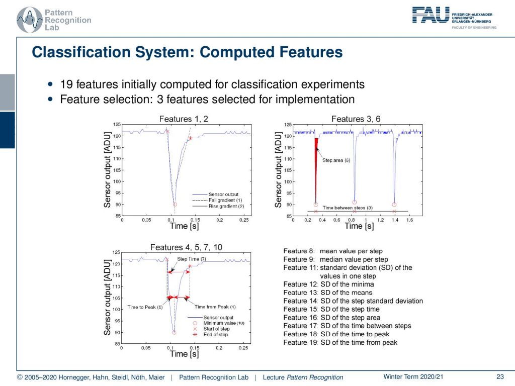
Concerning features, 19 features have been computed in this shoe for the classification. Then, in the end, only three features have been selected for implementation. The ideas of these feature computations are essentially an analysis of the step signal and the change of the cushioning material. So you need to detect when a step is performed. You can then derive from the amount of the change of the cushioning element, how hard the actual impact on the surface is. And you can also see on the steepness how the material that you’re running on or the entire system is reacting. From this, you can then control the stiffness of your shoe.
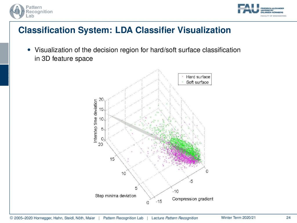
We can also visualize this in a three-dimensional space because we have three features. Here you can see the hard and the soft surface classes. You see that they form here approximately Gaussian classes, so we can very nicely apply our theory now. So we get the decision boundary, and then we simply decide we are on one side or the other side of the decision boundary here in this case. This is a very nice application of the LDA classifier in practice in an embedded system with very tough compute constraints.
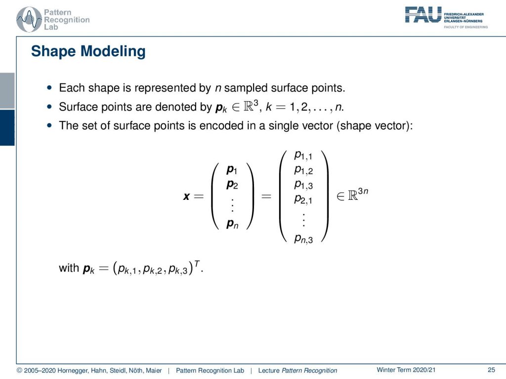
Another idea that I want to show you here in this context is shape modeling. Here the idea is that we sample surface points of a shape. So this is a 3D shape, and in particular, we’re interested here in the modeling of anatomical structures such as organs the liver, kidneys, lungs, and so on. We can sample them as surface points. So we take a fixed number of points for every shape. These are typically three-dimensional points, and we have a total of n points. Then we can encode the surface, given that we have the correct ordering of the points, into a single vector. So we write this up as a high dimensional vector that is then containing all of the elements of the 3D points. And this is then living in a space that has the dimension of three times n, where n is the number of points. So this is a very high dimensional space. Now, this is difficult to model, and you want to be able to model the degrees of shape changes according to anatomy in different patients.
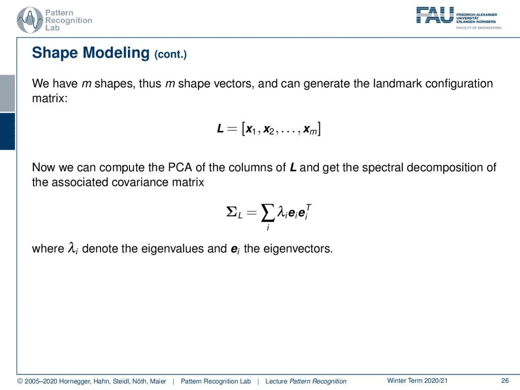
Now the idea that we have is that we have some m shapes, and this means that we have m shape vectors that give us this landmark configuration. So here, our vector x each has the dimension of three times n, and we have a total of m observations. This then allows us to compute a PCA of L and get the spectral decomposition of the associated covariance matrix. Here you can see that we essentially get the eigenvectors and associated eigenvalues. And if we sum them up, they would give again the respective covariance matrix. So this is essentially computed by using the principal component analysis here.
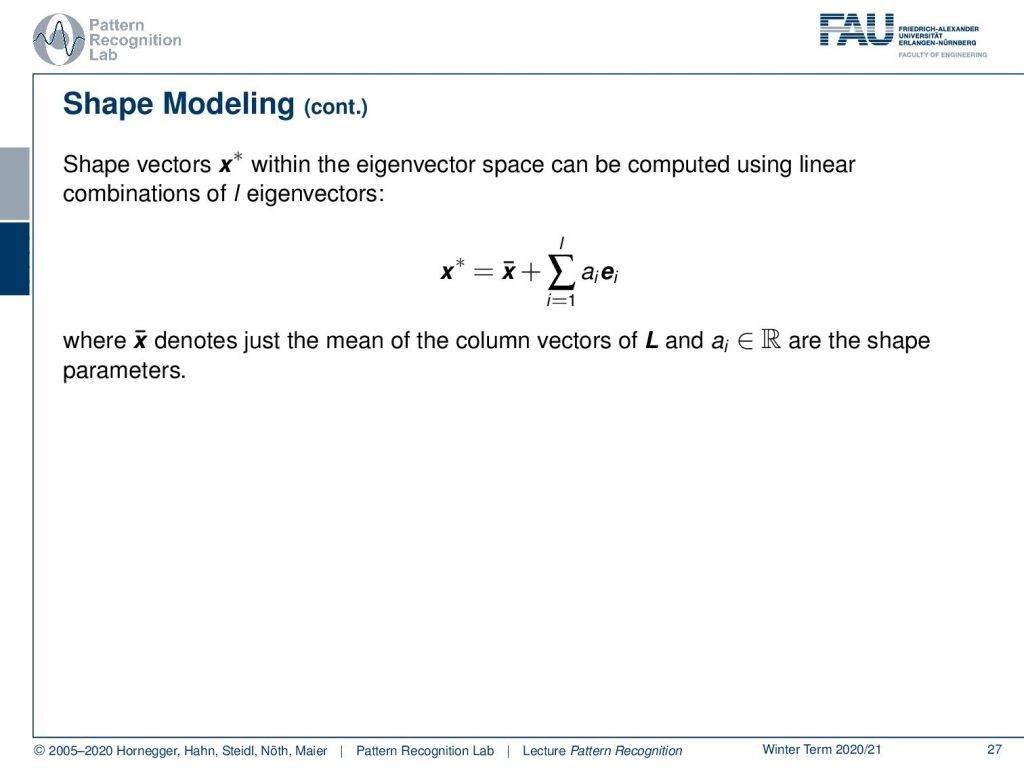
Now if we have that, then we can model all of our shapes with some x*, which is essentially giving us the shape configuration. The shape configuration can then be expressed as a linear combination of the eigenvectors. So we take the mean shape that is x̅, and x̅ is added on top of the number of chosen dimensions. Let’s assume we have the top three or top five modes of variation because they already explain let’s say 95% of the variance in the shape variations. Then we can use those, let’s say five, dimensions in order to express the most significant changes in the shape of these measures. Then we essentially end up with only five numbers that describe to us how the shape looks like.
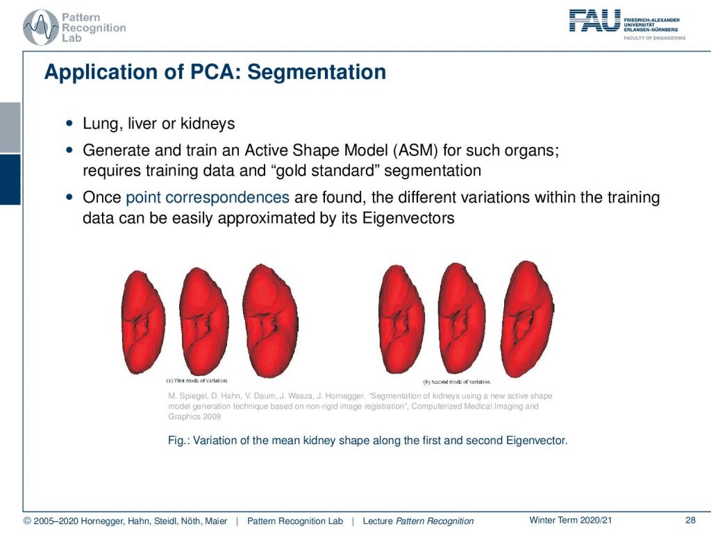
This is pretty cool, and it also allows us to model different shapes. Here we have, let’s say, a kidney. This kidney has different shapes and different patients, and we use the so-called active shape model then in order to generate the segmentation. The nice thing is now that we only have to estimate the rotation and translation with respect to the respective organ and the centroid in the volume. Then the shape can be described by very few parameters, as we’ve seen on the previous slide. Here, you essentially see the shape variations over the first two eigenvectors. On the left-hand side, you see the shape variations over the first eigenvector dimension, on the right-hand side the variation over the second eigenvector. So we can now use that and estimate rotation, translation, and those shape parameters.
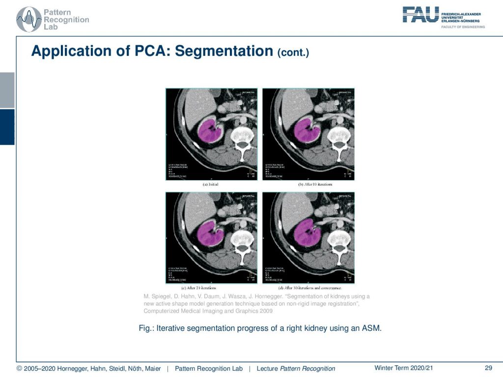
Here you see the fitting process over iteration. So we start with the mean shape that is here fitted into the kidney. And you see essentially a slice through the body. Also, we are indicating a slice through the mesh in purple. Over the iterations on the top right, bottom left, bottom right you can see how the change in shape parameters allows us to approximate the observed shape in the CT volume much better.
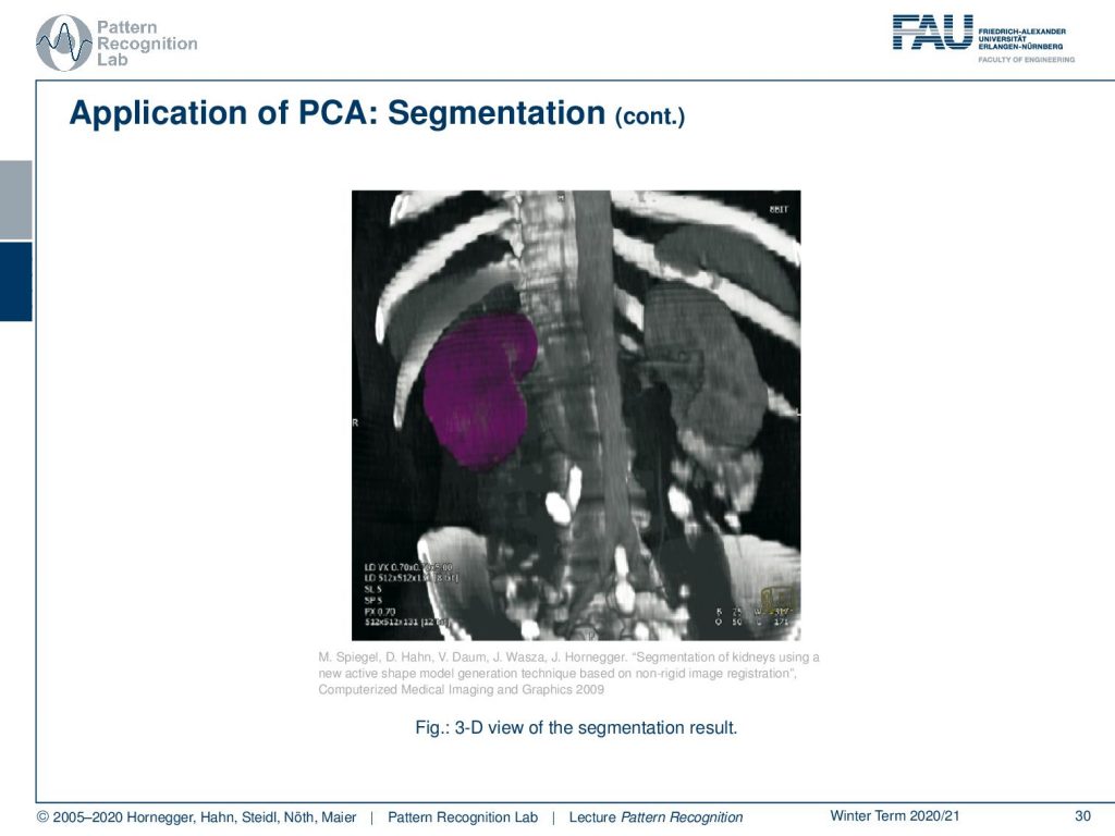
Then this yields a complete 3D segmentation of the kidney. This is a very popular method if you want to break down the complexity of shapes into a couple of dimensions. It allows you also then to sample plausible shape configurations from this shape model. So, PCA here is a very useful tool to describe the complex variations of anatomical changes in the body. If you got interested in this topic, please attend our lectures on medical image processing. There, we go into all of the details of the method how the active shape modeling search algorithm is performed, which transforms you have to perform on the image to make it work, and so on. So I can really recommend looking into these classes as well.

This already brings us to the end of this video. Next time in Pattern Recognition, we want to talk a little bit more about the general problem of regression and how regression can be regularized. This is a very important concept that we will also need in the next couple of videos. Thank you very much for listening and I’m looking forward to seeing you in the next video! Bye-bye.
If you liked this post, you can find more essays here, more educational material on Machine Learning here, or have a look at our Deep Learning Lecture. I would also appreciate a follow on YouTube, Twitter, Facebook, or LinkedIn in case you want to be informed about more essays, videos, and research in the future. This article is released under the Creative Commons 4.0 Attribution License and can be reprinted and modified if referenced. If you are interested in generating transcripts from video lectures try AutoBlog.
References
Lloyd N. Trefethen, David Bau III: Numerical Linear Algebra, SIAM, Philadelphia, 1997.
T. Hastie, R. Tibshirani, and J. Friedman: The Elements of Statistical Learning – Data Mining, Inference, and Prediction. 2nd edition, Springer, New York, 2009.
B. Eskofier, F. Hönig, P. Kühner: Classification of Perceived Running Fatigue in Digital Sports, Proceedings of the 19th International Conference on Pattern Recognition (ICPR 2008), Tampa, Florida, U. S. A., 2008
M. Spiegel, D. Hahn, V. Daum, J. Wasza, J. Hornegger: Segmentation of kidneys using a new active shape model generation technique based on non-rigid image registration, Computerized Medical Imaging and Graphics 2009 33(1):29-39