Lecture Notes in Pattern Recognition: Episode 37 – Adaboost Concept

These are the lecture notes for FAU’s YouTube Lecture “Pattern Recognition“. This is a full transcript of the lecture video & matching slides. We hope, you enjoy this as much as the videos. Of course, this transcript was created with deep learning techniques largely automatically and only minor manual modifications were performed. Try it yourself! If you spot mistakes, please let us know!
Welcome back to Pattern Recognition. Today we want to look into a particular class of classification algorithms and these are boosting algorithms that try to unite multiple weak classifiers into a strong one. Today we want to look into Adaboost.
So let’s have a look at the idea behind Adaboost. Boosting generally is trying to build a more powerful classifier from weak classifiers and you could say it is one of the most powerful learning techniques introduced in the last 20 years. It can be applied to any kind of classification system and you can get a bit of additional performance in any kind of situation where you really want to tweak out the last couple of percent in terms of performance. So the idea is to combine the output of many weak classifiers into a powerful committee. So it is essentially using the wisdom of the crowd and the most popular boosting algorithm is called Adaboost and was introduced in 1997.
So a weak classifier is one whose error is only slightly better than random guessing. But you need to have a classifier that is better than random guessing. Boosting won’t work with classifiers that are worse than random guessing. So the idea of boosting now is that you sequentially apply the weak classifier to repeatedly modified versions of the data and this produces then a sequence of classifiers. The weighted majority vote yields the final prediction.
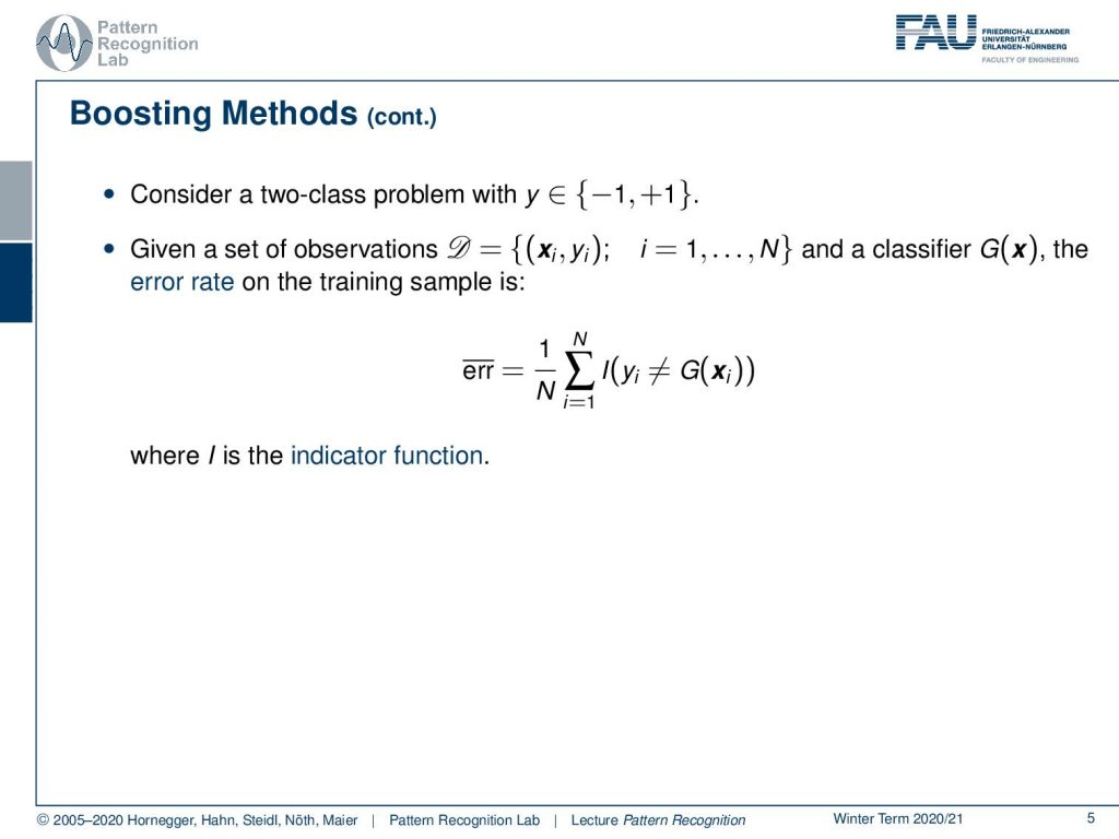
So we consider now a two-class problem with the class being either minus one or one and given some observations D that have a sample and a class. We can then train classifiers G(x) and this then implies that we also have an error on the training data set. This can be computed as the average error as 1 over n and then the sum over all the misclassifications where i is the indicator function which essentially checks whether this sample is true then it returns one otherwise zero.
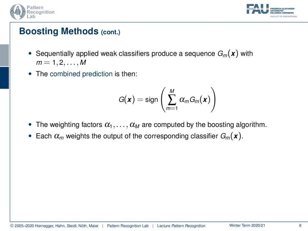
Now we can sequentially apply the weak classifiers to produce a sequence of Gm of these different weak classifiers. Then you can combine the weak classifiers in a sum and the final classification for G(x) is then given as the sign over the weighted sum of the individual classifiers. So we need some weighting factors α; α1 to αM. They are computed by the boosting algorithm. Then each α weighs the output of the corresponding classifier.
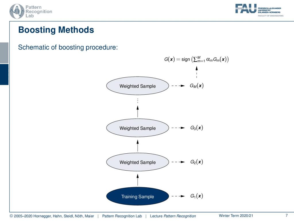
So you could summarize visually the boosting algorithm that you start with training some classifier. Then you compute the error on the training set, you re-weight the samples, train a new classifier, compute the error on the training set, re-weight the samples, and so on and so on until you then stop at some point where you have trained m classifiers.
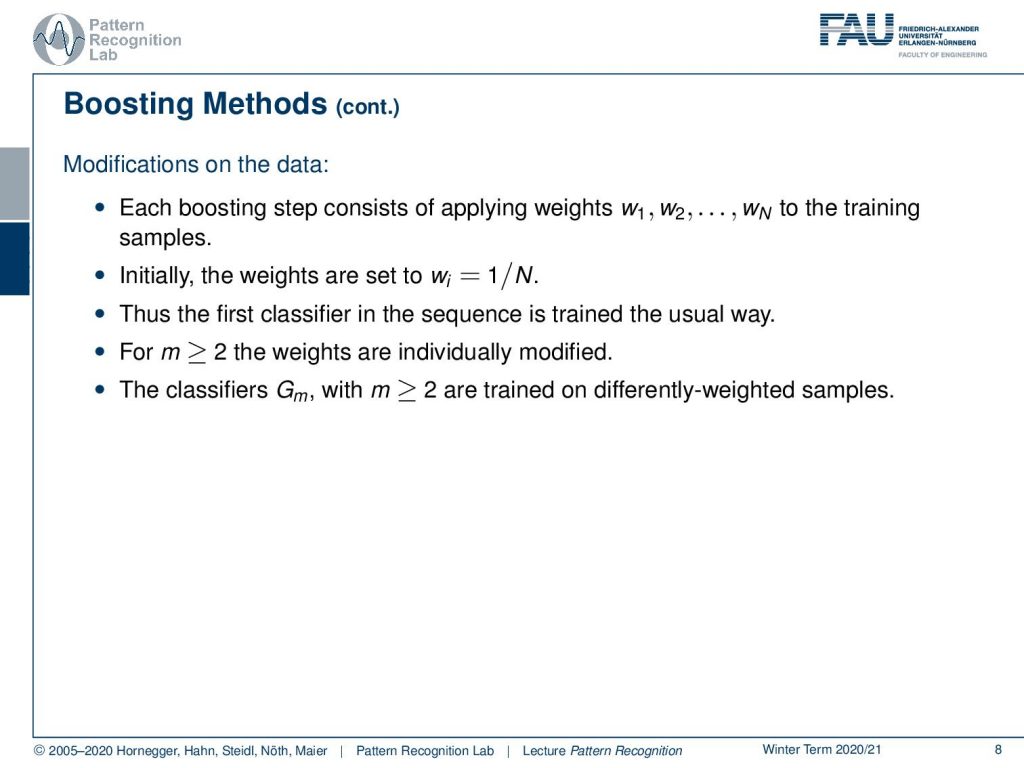
So each boosting step consists of applying the weights to the training samples that essentially amplify the weight of misclassified samples. Initially, you can start with the weights just uniformly distributed. So the first classifier in the sequence is trained just the usual way and then for m greater or equal to two the weights are then individually modified. Then the classifiers Gm with m greater or equal to two are trained on differently weighted samples.
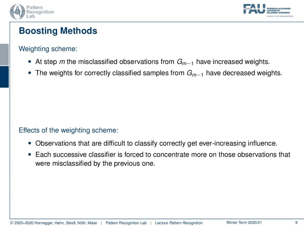
Now the waiting scheme at step m looks as the misclassified observations that have been produced by the previous classifier and there we have to increase the weights. The weights for correctly classified samples have decreased weights. So this then means that observations that are difficult to classify get ever-increasing influence over the iterations. Each successive classifier is forced to concentrate more on those observations that were misclassified by the previous one. This then brings us to the Adaboost iteration scheme.
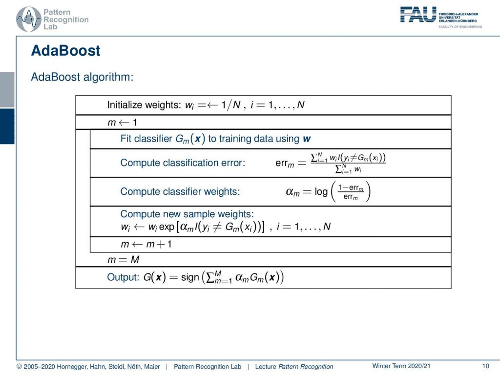
So you initialize your weights with a uniform distribution. Then you set the iteration counter to one. You fit the first classifier onto the training data set and you use the current weights. Then you compute the classification error that is essentially a weighted sum of the misclassifications. Then you update the classifier weights and here we use the classification error in order to guide us which classifier to trust more and which classifier to trust less. Then we can compute new sample weights again using our classification loss of our new joint classifier. This way we can then go ahead and iterate over and over again until we have built the desired number of classifiers in our example m. Then we finally output the completely trained classifier. So you see that in every iteration of Adaboost we have to train a new classifier.
So this version of AdaBoost is called the discrete version because each classifier returns a discrete class label. Adaboost can also be modified to return a real value projection in the interval from -1 to 1. Instead of just taking any classifier for Gm the classifier may be used that results in the smallest error at step m. So Adaboost dramatically increases the performance even of a very weak classifier and we can do this by looking at some examples.
So this is from the Technical University of Prague, from where we essentially got the data to generate those plots. If you just start with a single linear decision boundary, you see that this problem cannot be solved. You will get something like this and this is of course not a very good solution. But it will kind of perform better than a random classification. Now this gives us the following misclassified samples and now because we were able to construct the misclassified set, we are now able also to compute updated weights for the next iteration.
Now let’s have a look at how this behaves over the training process where we start in our first training with this simple perceptron classifier. You see that we have a rather high training error. Now we do a second iteration you see that the error is already slightly reduced. Then in the next iteration, we have a dramatic reduction of error. Then we have another sample that is added error goes up but with another plane that is added the error goes down again. Now we can iterate this until we end at the desired number of classifiers of m and you can see that the center is now very well classified towards the correct class. We still have some outliers at the boundaries but generally, this has a very good classification performance only using linear decision boundaries on this problem that can typically not be solved with a linear decision boundary.

So next time in pattern recognition we will look a little bit more into the mathematical details of Adaboost and in particular, we want to look at the exponential loss function. So I hope you enjoyed this little video and I’m looking forward to seeing you in the next one.
If you liked this post, you can find more essays here, more educational material on Machine Learning here, or have a look at our Deep Learning Lecture. I would also appreciate a follow on YouTube, Twitter, Facebook, or LinkedIn in case you want to be informed about more essays, videos, and research in the future. This article is released under the Creative Commons 4.0 Attribution License and can be reprinted and modified if referenced. If you are interested in generating transcripts from video lectures try AutoBlog
References
- T. Hastie, R. Tibshirani, J. Friedman: The Elements of Statistical Learning, 2nd Edition, Springer, 2009.
- Y. Freund, R. E. Schapire: A decision-theoretic generalization of on-line learning and an application to boosting, Journal of Computer and System Sciences, 55(1):119-139, 1997.
- P. A. Viola, M. J. Jones: Robust Real-Time Face Detection, International Journal of Computer Vision 57(2): 137-154, 2004.
- J. Matas and J. Šochman: AdaBoost, Centre for Machine Perception, Technical University, Prague. ☞ http://cmp.felk.cvut.cz/~sochmj1/adaboost_talk.pdf