Lecture Notes in Pattern Recognition: Episode 34 – Measures of Non-Gaussianity

These are the lecture notes for FAU’s YouTube Lecture “Pattern Recognition“. This is a full transcript of the lecture video & matching slides. We hope, you enjoy this as much as the videos. Of course, this transcript was created with deep learning techniques largely automatically and only minor manual modifications were performed. Try it yourself! If you spot mistakes, please let us know!
Welcome back to Pattern Recognition! Today we want to explore a little bit more ideas about the independent component analysis ICA. We’ve seen so far that the Gaussianity or Non-Gaussianity is an important property of independent components. In today’s video, we want to look into different measures of how to determine this Non-Gaussianity.
We’ve seen that the key principle in estimating the independent components is non-Gaussianity. To optimize the independent components we need a quantitative measure of non-Gaussianity. Furthermore, let’s consider our random variable y and assume that it has zero mean and unit variance. Of course, we enforce this already by appropriate pre-processing. Now we will consider three measures of non-Gaussianity and we’ll look into the kurtosis the negentropy and mutual information.

Let’s start with the Kurtosis. The definition of Kurtosis is the expected value of y4 minus 3 times the square of the expected value of the power of two of the original signal. If we have unit variance and zero mean you can see that this simplifies to the signal to the power of 4 and then you subtract 3 because we simply have the covariance matrix as the identity matrix. Then this essentially gives us just a factor of 3. Now if you have two independent random variables y1 and y2, then linearity properties hold. This means that the kurtosis of y1 plus y2 is going to be given as the kurtosis of y1 and the kurtosis of y2. Also, scaling with a factor of α would then result in the kurtosis of y multiplied with the factor α4. Now here α is a scalar value.
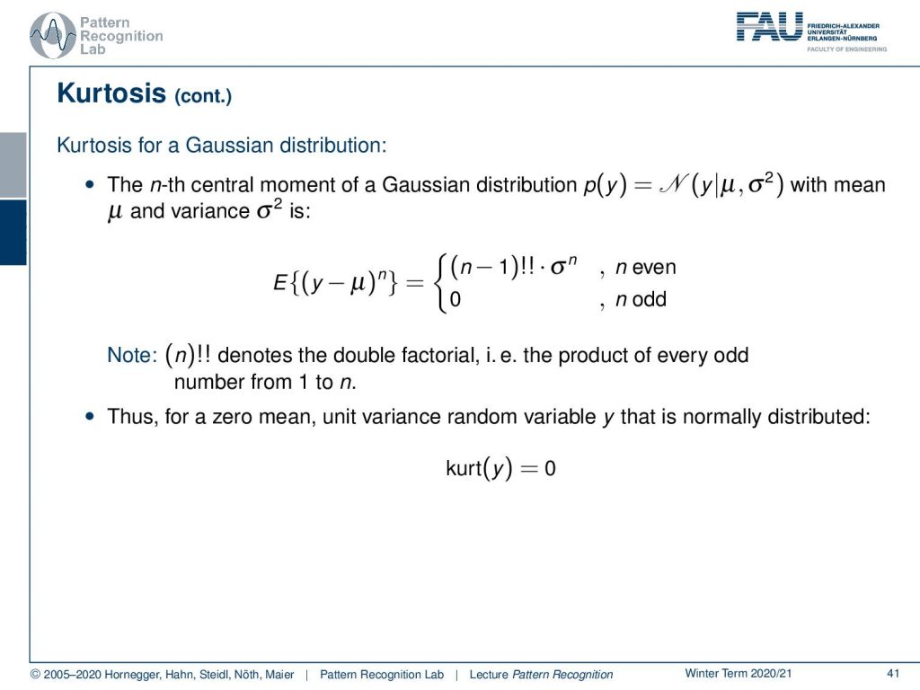
Let’s have a look at the Kurtosis for a Gaussian distribution. The n-th central moment of a Gaussian distribution with p(y) equals to the normal distribution with mean y and variance σ2 can then be determined as the expected value of y minus μn. You will see that this is going to be (n-1) double factorial times σn if n is even and 0 if n is odd. So for your 0 mean and unit variance random variable y that is normally distributed we will have a Kurtosis of zero.
The Kurtosis is zero for a Gaussian random variable with zero mean and unit covariance. For most but not all non-Gaussian random variables the Kurtosis is non-zero. So the Kurtosis can also be positive or negative. Typically, then the non-Gaussianity is measured as the absolute value of the Kurtosis or the Kurtosis to the power of two.
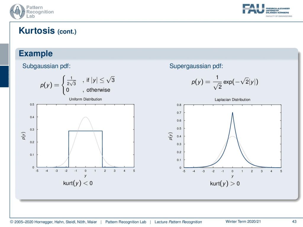
Let’s look into a Subgaussian probability density function. Here we choose the uniform distribution. You can see that in this case, the Kurtosis is going to be negative. If we have a Supergaussian probability density function, for example, we take the Laplacian distribution, then you will see that the Kurtosis is greater than zero.
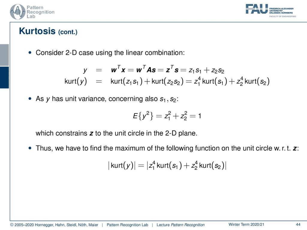
If you consider the 2D case using a linear combination, then you can see that we can express our y as wTx. Now we replace x with the mixing matrix and the original signals. Then we can rewrite the weighting vector as this inner product with z and s. If we have two variables we can write this as z1 times s1 plus z2 times s2. Then the kurtosis of y would be given as the Kurtosis of z1 times s1 plus the Kurtosis of z2 times s2. And this can be rewritten using our scalar property as z14 times the kurtosis of s1 plus z24 times the kurtosis of s2. So as y also has a unit variance concerning s1and s2 we can now write up the expected value of y2. You see that this is going to be given as z12+z22. This is supposed to be 1 because of our scaling, so this constrains our set to the unit circle in the 2D plane. Now we have to find the maximum of the function on the unit circle concerning z. The absolute value of the Kurtosis is given by the absolute value of the reformulated Kurtosis for the two signals.
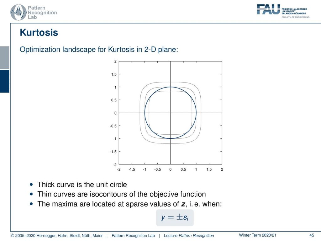
And here we have a couple of examples for the landscape of the Kurtosis in a 2D plane. Here the thick curve is the unit circle and then the thin curves are isocontours of the objective function. You see that the maxima are located at sparse values of z. And, for example, you find them where y is +-si.
How would we maximize the non-Gaussianity of a vector w in practice? You start with some initial vector w, then you use gradient descent to optimize the maximization of the absolute value of the Kurtosis. And of course, you want to do that after transforming with w so you plug this in here. Then you plug this optimization into the ICA estimation algorithm that we’ve seen in the previous video.
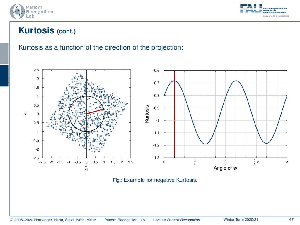
Let’s visualize the Kurtosis as a function of the direction of the projection. Here you can see that you get this repeating structure in our example. The maximal direction here is indicated with the red line and the right-hand plot where we see the function of the Kurtosis for the angle. Or we also indicate this direction in the left-hand plot with the red line. We see the maximal Kurtosis for the super-gaussian projection directions and the minimal Kurtosis for the sub-gaussian projection directions.
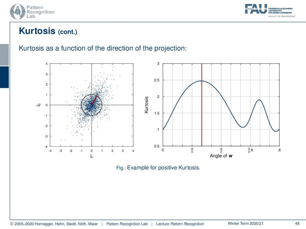
Let’s look at an example with only positive Kurtosis. Here we have a noisy distribution. And again, we indicate the maximum direction using this red line here. You can see now that we are essentially able to determine one major lobe of the distribution. Still, we see a small maximum as a kind of second lobe. So you see that it can identify independent components, but it also has some problems in identifying noise as an additional component.
Now we see that kurtosis is a valid measure for non-Gaussianity but it has some drawbacks in practice, in particular when it’s computed on a set of measurement samples. So the Kurtosis can be very sensitive to outliers due to the higher-order statistical moments. It’s not optimal for supergaussian variables, even without outliers as we’ve seen in the example. And it is not a robust measure of non-Gaussianity.
Let’s look into some different ideas! The next one is Negentropy. A Gaussian variable has the largest entropy among all the variables of equal variance. We’ve seen that already. So entropy is essentially a measure for the distributions that are spiky. Negentropy can thus be used as a measure for non-Gaussianity, it is zero for the Gaussian random variables and always non-negative. The Negentropy can then be defined for a variable y as the difference between the entropies of a Gaussian distribution with the same covariance and mean vector and the distribution under consideration.
The properties of Negentropy are that it’s a measure that is justified well by statistical theory. In theory, Negentropy is an optimal statistical estimator of non-Gaussianity. Furthermore, computing the Negentropy from a measured set of samples requires essentially an estimation of the probability density function. And, as you may know, the non-parametric estimations of a pdf from samples is non-trivial and often computationally quite expensive. There you have to use approximations for Negentropy, and there are ones that are robust and computationally more efficient than the direct pdf based approaches.
Let’s look into a third approach that is mutual information. This is our information-theoretic approach. The Negentropy measures the difference in terms of information value to Gaussian random variables. Instead, we could measure the statistical dependence between the random variables directly. So the mutual information is a concept to measure the entire dependency structure of random variables and not only the covariance.
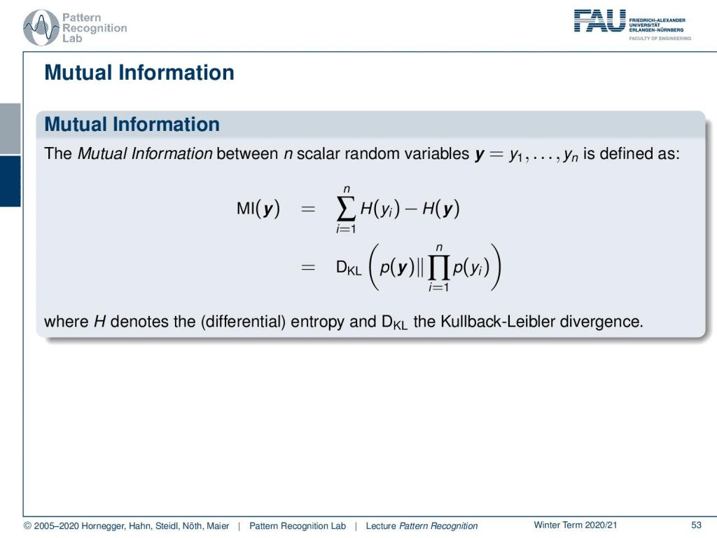
The mutual information can be computed between n scalar random variables y that is y1 one to yn as a sum over the differences in entropy. This is identical to computing the KL divergence of the joint probability density function with the probability density functions where we assume that the individual components are mutually independent. So we can simply write this as a product over the component-wise probabilities. Again here H denotes the differential entropy and DKL is of course the Kullback-Leibler divergence.
Our interpretation here is that entropy can be regarded as a measure of code length. And then H(yi) is a measure for the code length necessary to encode yi. So if we now look at H(y), it can be regarded as the code length necessary to encode the entire vector y. In this context, the mutual information shows the reduction in code length obtained when encoding y instead of the components of yi separately.
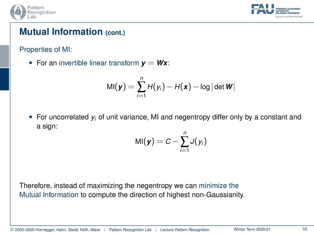
There are also several important properties of mutant information. For an invertible linear transform y=Wx, we can write the mutual information as the sum over the entropy of yi minus the entropy of x minus the logarithm of the determinant of W. For uncorrelated yi of unit variants, the mutual information and neck entropy differ only by a constant and a sign. You see if the signals are uncorrelated and of unit variance, you can express the mutual information as the Negentropy. Therefore, instead of maximizing the Negentropy, we can minimize the mutual information to compute the direction of the highest non-gaussianity.
What are the lessons that we learned here in ICA? ICA is a simple model based on linear non-Gaussian latent variables. And we see by mixing these non-Gaussian latent variables we create something that is more Gaussian. So the non-Gaussianity is a key principle in order to compute the separation matrix. We estimate this by maximizing the non-Gaussianity of the independent components. We’ve also seen that we can equivalently use Kurtosis, Negentropy, and mutual information to measure the non-Gaussianity.

Next time in Pattern Recognition we want to have a look at the No Free Lunch theorem and also the bias-variance trade-off which are very important concepts when you think about actually finding the optimal classifier and which model is best suited for your classification task at hand.
Of course, I also have some further readings. If you want to read more about independent component analysis there is this wonderful paper “Independent Component Analysis: Algorithms and Applications”. And you can also find something about this in “The Elements of Statistical Learning”, as well as in “Elements of Information Theory”.
I also have some comprehension questions for you that may help you with the preparation for the exam.
And this brings us to the end of this video. I hope you enjoyed this little excursion into different measures of non-Gaussianity and I’m looking forward to seeing you in the next video! Bye-bye.
If you liked this post, you can find more essays here, more educational material on Machine Learning here, or have a look at our Deep Learning Lecture. I would also appreciate a follow on YouTube, Twitter, Facebook, or LinkedIn in case you want to be informed about more essays, videos, and research in the future. This article is released under the Creative Commons 4.0 Attribution License and can be reprinted and modified if referenced. If you are interested in generating transcripts from video lectures try AutoBlog.
References
- A. Hyvärinen, E. Oja: Independent Component Analysis: Algorithms and Applications, Neural Networks, 13(4-5):411-430, 2000.
- T. Hastie, R. Tibshirani, J. Friedman: The Elements of Statistical Learning, 2nd Edition, Springer, 2009.
- T. M. Cover, J. A. Thomas: Elements of Information Theory, 2nd Edition, John Wiley & Sons, 2006.