Lecture Notes in Pattern Recognition: Episode 33 – Independent Component Analysis and Gaussianity

These are the lecture notes for FAU’s YouTube Lecture “Pattern Recognition“. This is a full transcript of the lecture video & matching slides. We hope, you enjoy this as much as the videos. Of course, this transcript was created with deep learning techniques largely automatically and only minor manual modifications were performed. Try it yourself! If you spot mistakes, please let us know!

Welcome back to Pattern Recognition. Today we want to look a bit more into the Independent Component Analysis and in particular, we want to think about what it actually means if the components are independent. 

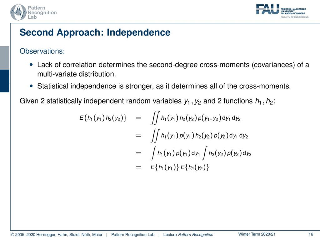
Now let’s build on the previous ideas. So you can see that using the Whitening transform we were able to uncorrelated the signals but the correlation is only determined by the second degree cross moments, the covariances of a multivariate distribution. Now statistical independence is a much stronger statement than correlation as it determines all of the cross moments. So this then means that if we have two statistically independent variables y₁ and y₂ and two functions h₁ and h₂ we can have a look at the expected value of the multiplication of the two. So you could say h₁ and h₂ is the mixing and you could say y₁ and y₂ are the actual signal sources. Now you can see I can write up this expected value as the double integral over h₁ of y₁ times h₂ of y₂ times the joint probability of y₁ and y₂ appearing together. Now we assume independence which means that we have the joint probability expressed as the product of the individual probabilities and this then allows us to split the joint probability and if we do so we can also split the integral into two integrals. Now you can see that the two remaining integrals only focus on one of the two variables which means that I get the product of the expected values. 

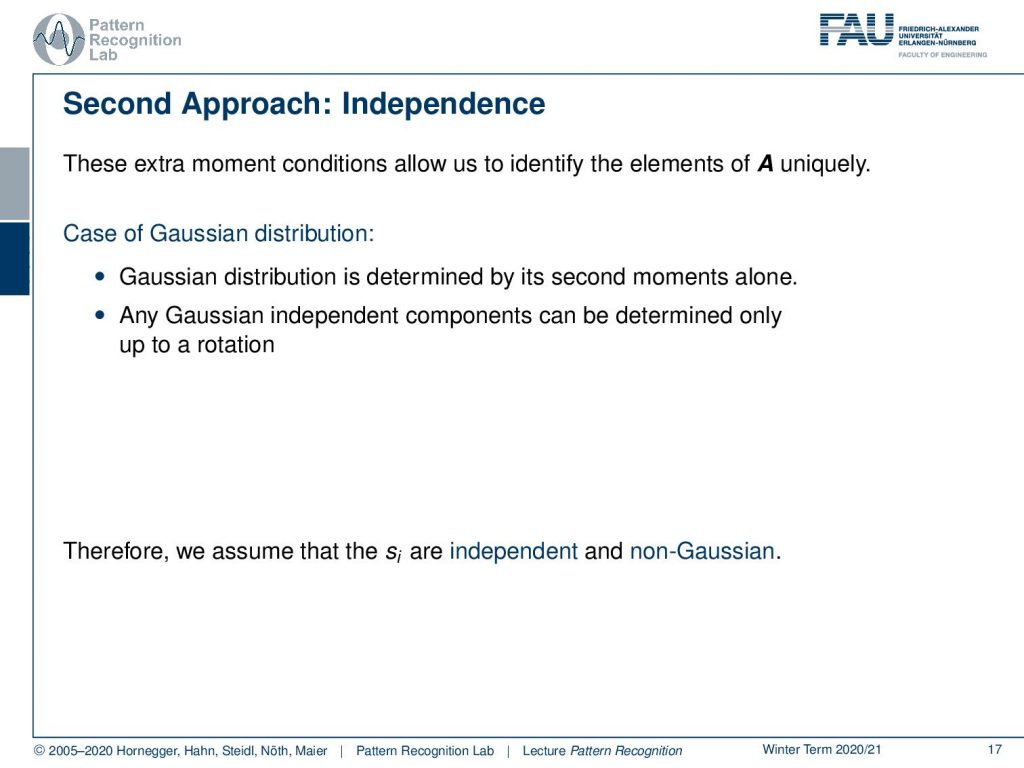
So the extra moment conditions allow us to identify the elements of A uniquely. So we do more than de-correlation. In the case of a gaussian distribution, this is not the case because it is determined by its second moments alone. So in a Gaussian distribution, you don’t need the additional moments because if you have the mean and the covariance matrix you have already determined the Gaussian distribution. So any gaussian independent components can be determined only up to a rotation. Therefore we assume that the s_i is independent and we assume that they are non-gaussian because if they are gaussian our independent component analysis would simply not work. 

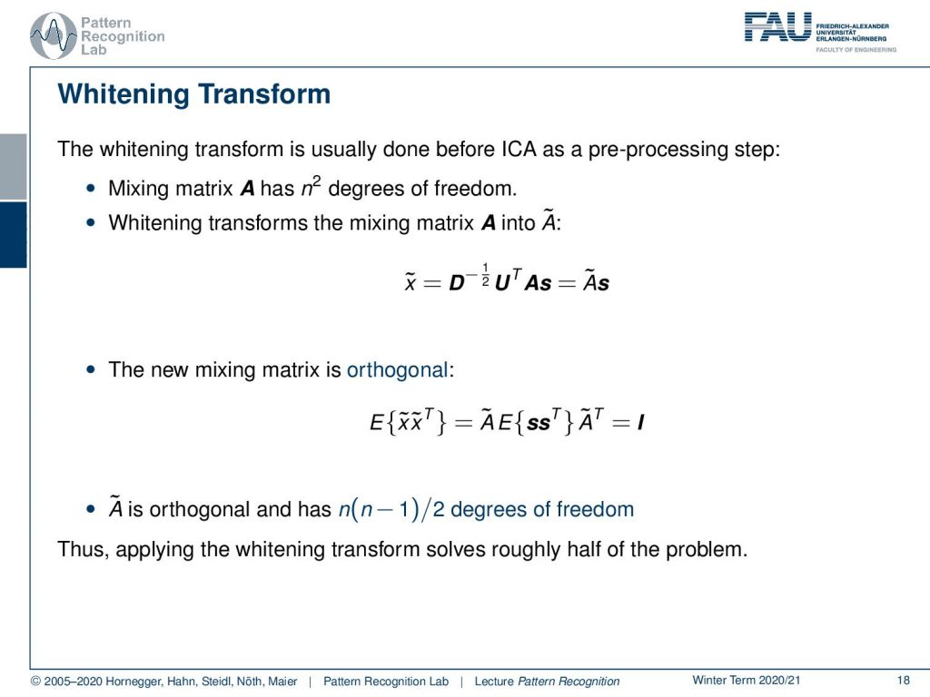
If you look at the Whitening transform then this is typically a pre-processing step of our process. So you would have this observation that the matrix A typically has n to the power of 2 degrees of freedom. Now if you apply the Whitening transform first you can actually see that we only need to consider the transformed feature space. So here x̃ is the transformed one and then we would apply our mixing matrix. So we can essentially write this up as some àwhich is essentially the matrix that does the whitening transform and mixing together. Now the new mixing matrix is orthogonal you can discover this if you look at the expected value of x̃, x̃ transpose so you look at the covariance matrix. We know our independent component analysis is supposed to map onto our independent signals. So we can pull out our àand àtranspose on both sides. Then you can see that this expected value of the signal and the signal transpose is nothing else than the covariance matrix of our signals. They’re independent, so this is going to be the identity matrix. Now you just have àtimes àtranspose and this has to map to the identity matrix and therefore we can see that it’s going to be an orthogonal matrix. So àis orthogonal and it has n times n minus 1 over 2 degrees of freedom and thus applying the whitening transform already solves half of the problem. So we can simplify the problem and we already get a step closer to our solution.

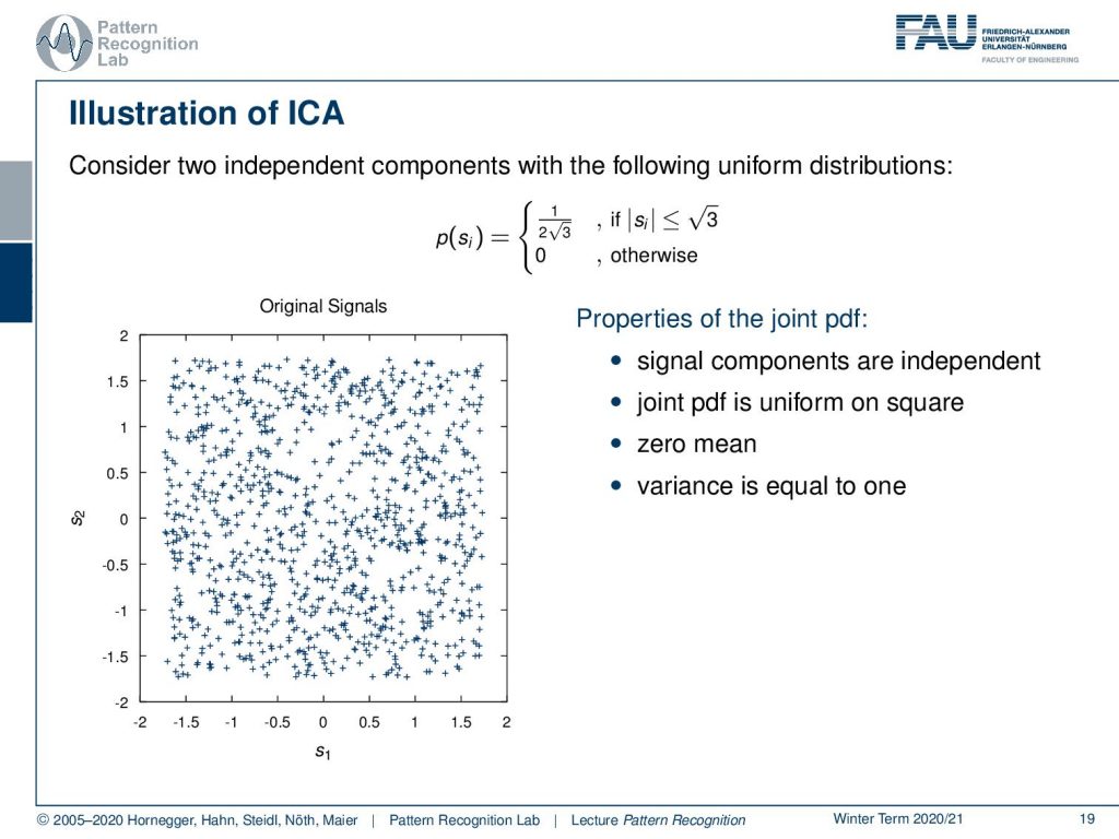
So let’s have a look at the ICA and find an illustration. So here we’ll have two uniform distributions that we want to show and they are essentially mapping onto an equal probability that is determined within the interval of plus and minus square root 3. If you do so then you get essentially a distribution like this one. So you are uniformly distributed and independently distributed on both dimensions. Then the joint probability is uniform on a square. This also has zero mean and the variance is equal to one. So these are our signals and let’s mix them.

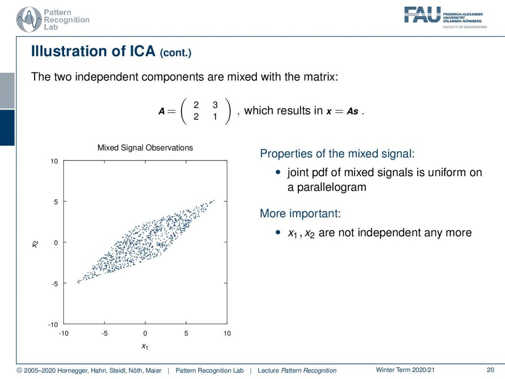
If we mix them we can set up a mixing matrix and here we just choose the matrix A as 2, 3, 2, 1 and now we can compute x. If we do so we get the following result for the mixed observation. So you can see that our square has been transformed into this diamond. Now the joint probability density function is essentially a uniform distribution on a parallelogram. More important is even that the x₁ and the x₂ are not independent anymore. 

Now let’s try to estimate A. So the edges of the parallelogram are the directions of the columns of A. In principle, we could first estimate the joint probability density function of x₁ and x₂ and if we locate the edges of the joint probability density function, we can estimate A. But this is computationally very expensive and this principle only works exactly with uniform distributions. We want to be able to process any kind of non-gaussian distribution. So this is not the solution scheme that we would do in general. But it is able to capture the non-gaussianity of the distribution and then apply this in our independent component analysis.

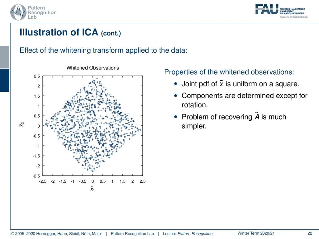
Let’s see what our Whitening transform does. If we apply Whitening transform to our data it would map onto the following space. So this is x̃₁ and x̃₂ and you can see here that the joint pdf of x̃ is uniform on a square. The components are determined except for the rotation. So we are missing the correct rotation to map back onto our independent components. so the problem of recovering àis much simpler than the recovery of the original mixing coefficients. 

So we see that in the ICA model we need to assume that the s_j are mutually independent. Also, the s_j has to be non-gaussian in order to be able to determine them from the x_i. For simplicity, we assume that our A is square and then we still end up with some ambiguities. For example, the s_j is determined only up to a multiplicative constant and the s_j is not ordered. 

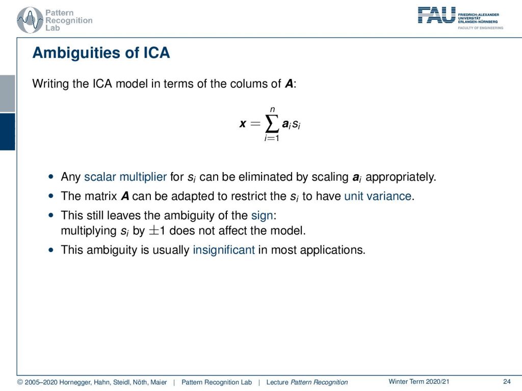
So let’s see why this is the case. So you can see that the observation that we are actually getting is essentially a sum over the column vectors of A and they are multiplied with the strength of the respective signal. This also means then that any scalar multiplier for s_i here can be eliminated by scaling a_i appropriately. So we can get rid of this problem of not being able to determine the scaling because we could for example propose to restrict the matrix A such that it will perform a scaling towards a unit variance. But this still would leave the ambiguity of the sign. So if you multiply by plus one or minus one it would not affect the model. So you would still have the unit variance it would just be flipped. Typically this ambiguity is usually insignificant in most applications because if you know how the signal is supposed to look you can use a prior in order to figure out this ambiguity. So for example, if the gray values of your image are flipped then you can very easily correct that by multiplying with -1. You can very easily determine whether you have reconstructed the negative or the true image just by looking at the data.

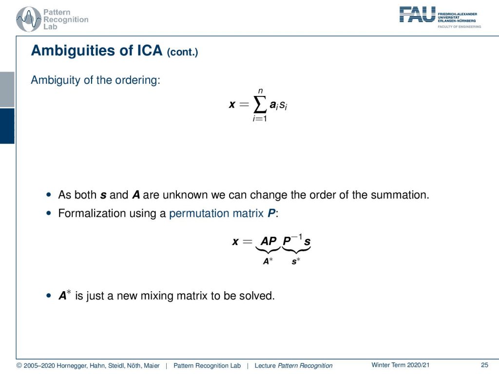
There is also the ambiguity of ordering. So here you see that we sum up over the columns and as s and a are unknown we can change the order of summation. This is then typically formalized by using a permutation matrix. This permutation matrix is then reordering the entire sum. This means that A* would simply be a new mixing matrix that needs to be solved. So generally we cannot determine a sequence in the independent component analysis because of this effect. So if you did the unmixing then you still have to identify which source was actually mapped onto which channel. So this is a general drawback of ICA and you have to do it. Again you can use prior knowledge in order to figure out which channel is mapped onto which output of the ICA. 

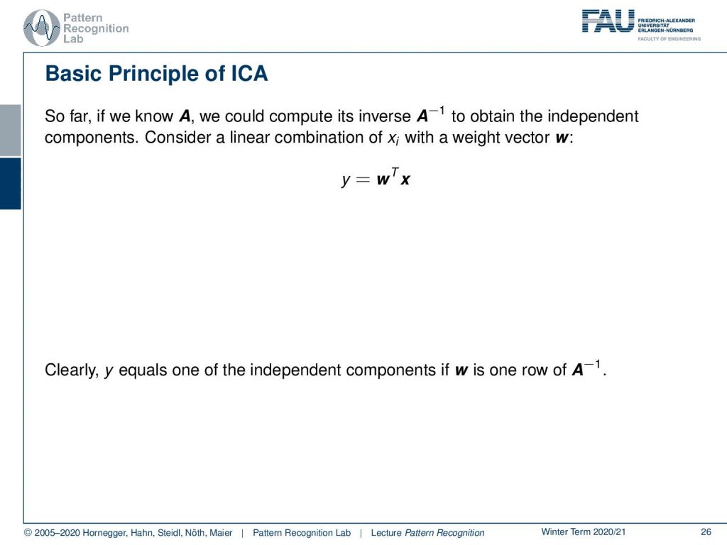
So far if we know A we could compute the inverse of A in order to obtain the independent components. So if you consider a linear combination of x_i with a weight vector w you could see that we could now express some y as the inner product of the vector w with x. Then clearly y equals to one of the independent components if w is one row of A inverse. So we can use this in order to perform a change in variables. So now let’s map to some variable set and set is determined as A transpose w and then you can apply this in the linear combination. So you get y equals to w transpose x. 

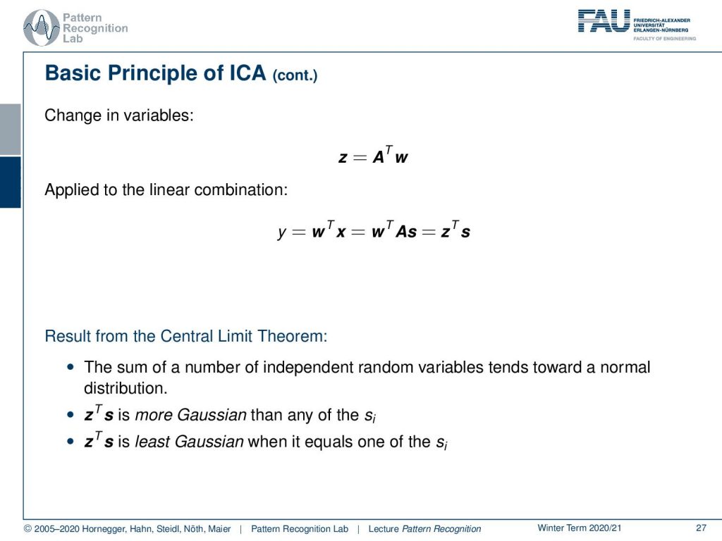
Now we do the substitution. So we have w transpose A times s and this can then be rewritten as z transpose s. Now we know the result of the central limit theorem. The sum of many independent random variables tends towards a normal distribution. So you could say x transpose s is more gaussian than any of the individual components s_i. So z transpose s is going to be least gaussian when it equals to one of the independent components s_i. 

This leads us now to the key principle of the independent component analysis. We maximize the non-gaussianity of w transpose x and this will then result in the independent components.

So if you have a look at the marginal distributions of the joint and the mixed-signal then you can see that if we have this kind of distribution so for s₁ and s₂ and we compute the marginal of the joint probability. You can see now that for s₁ we get essentially this distribution and you see that it is close to the uniform distribution as we have defined the problem. Now we can do the same thing with the marginal distributions of the mixed observations. Here you see that if we do the same computation then we suddenly end up with something that looks much more gaussian. So you see that the mixing of the independent components increases their gaussianity. 

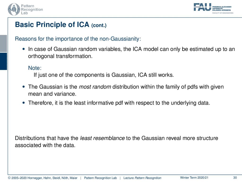
So this brings us then to the reasons for the importance of non-gaussianity in the case of Gaussian random variables. The ICA model can only be estimated up to an orthogonal transform and by the way, if just one of the components is gaussian the ICA will still work. The gaussian is the most random distribution within the family of probability density functions with given mean and variance. Therefore it is the least informative probability density function with respect to the underlying data. So distributions that have the least resemblance to the gaussian reveal more structure associated with the data. 

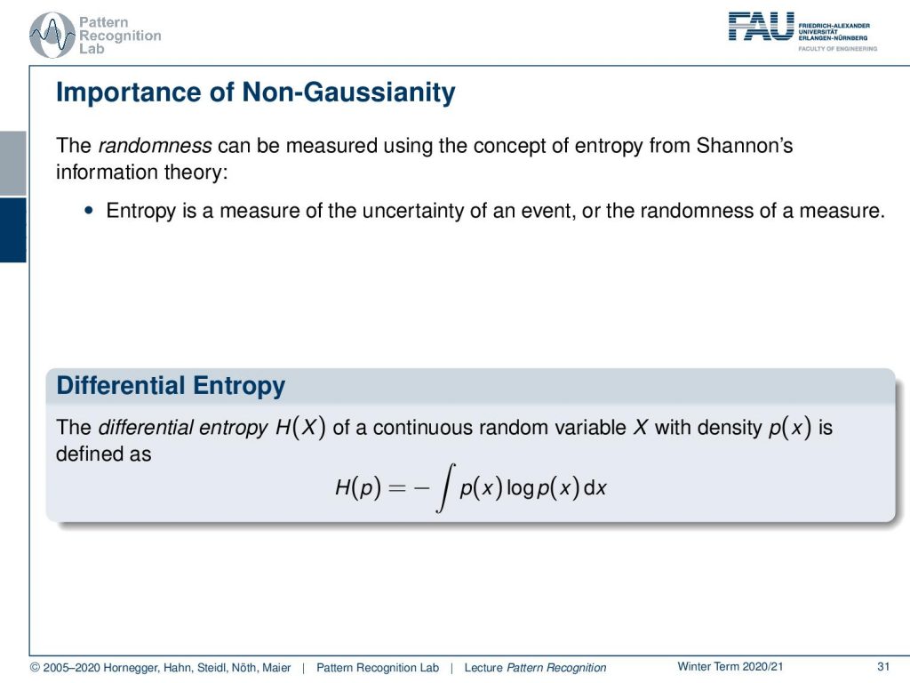
So let’s have a look at the importance of non-gaussianity. The randomness can be measured using the concept of Shannon’s information theory. We do that by computing the entropy because the entropy is a measure of uncertainty of an event or the randomness of this measure. The differential entropy of a continuous random variable x with density p(x) can be found as h(p) equals to minus the integral over p(x) times the logarithm of p(x) integrated over x. 

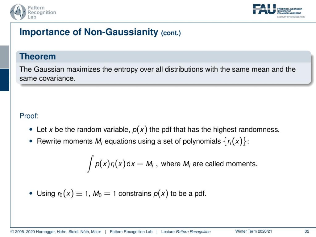
Let’s have a look at this theorem. The gaussian maximizes the entropy over all distributions with the same mean and the same covariance. We can actually prove this so let x be the random variable p(x) the pdf that has the highest randomness. Then we can also rewrite the moments’ M_i equations using a set of polynomials. So you see here where we introduce this as an integral of the pdf multiplied with some r_i and this then results in the moments. Now we can see if we choose the rs appropriately we get the moments. So here we choose the r0 to be always 1 and this then results in M₀ which is going to be exactly 1, which is the sum over the entire probability density function. Now, this constrains p(x) to be a probability density function, otherwise, we can now use polynomials in r and these polynomials can then be used in order to determine the moment. You see that these will then be the mean the standard deviation and so on. 

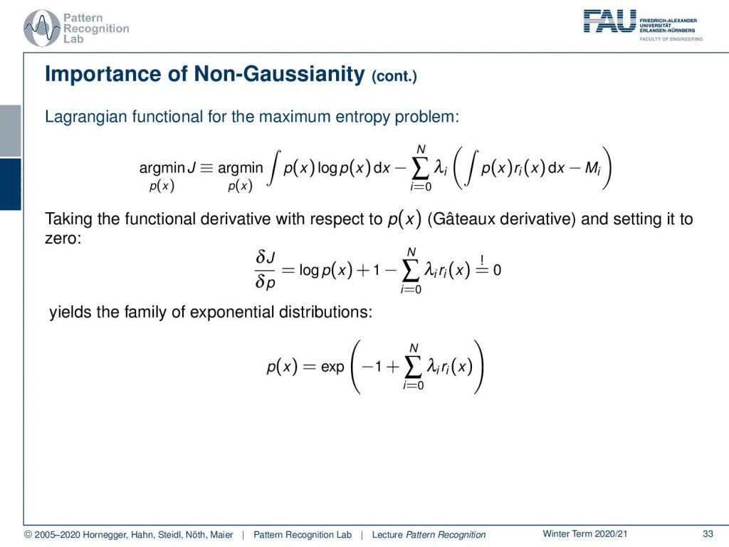
Now if we go ahead then we can put that into a Lagrangian formulation for maximizing the entropy. So we start with the entropy and we constrain this entropy with our Lagrange multipliers. You see here that the respective moments need to equal exactly the moments that we have determined. Now we can take the functional derivative with respect to p(x) which is the cathode derivative and set it to zero. Here you see then that our minimization with respect to p is going to be found as the logarithm of p(x) plus one minus the sum over the individual polynomials that are determined to construct the moments. This essentially then yields the family of exponential distributions. 

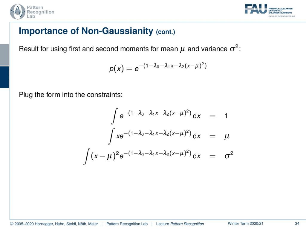
Now let’s look at the first and second moments to be given by mean μ and variance σ square. Then you can see that we can write this up in the following polynomial form. So this essentially breaks down to e to the power of minus and then 1 minus λ₀ minus λ₁x minus λ₂(x – μ² ) and now we plug this into our constraints. Here you see that the moments have to be determined by this and you see here then that you get these three constraints. So the zeroth moment needs to fulfill the property that is a probability density function. So the integral over the entire function needs to be one. The first moment is going to be given by the mean value and the second moment is going to be given by the sigma square. 

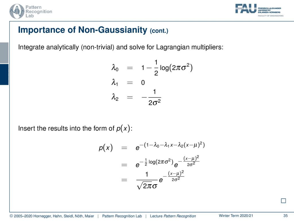
Now we can solve this and this is actually non-trivial but if we solve for the Lagrangian multipliers we get the following observation. We get λ₀ equals to 1 minus 1 over 2 and the logarithm of 2πσ², λ₁ is 0 and λ₂ is minus 1 over 2σ². Now we insert this into our probability density function and rearrange this a little bit and you see we get exactly the gaussian distribution. So the Gaussian distribution is the distribution that maximizes the entropy with given mean and variance. 

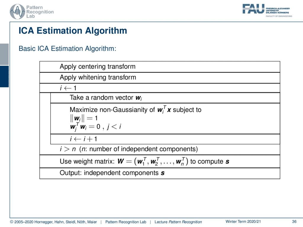
Now let’s look at how we would then construct such an ICA algorithm. So we would apply a centering transform. We would apply the Whitening transform and then we start iterating we take a random vector w_i and then we maximize it with respect to non-gaussianity of wi transpose x subject two that the length of the vector is one and the inner product of any other w_j with respect to w_i is going to be zero. Then we can increase the iteration counter and we do that for all our independent components. Then we can use this weight matrix once we have determined it in this iterative process and compute the independent signals using exactly this transform. The final output is then the independent components s.

So now let’s look at a couple of nodes in this process the estimation is steered by maximizing the non-gaussianity of independent components. There exist equivalent algorithms for solving the ICA. They’re gradient descent methods and there are things like fast ICA. There is even a relation to projection pursuit that was introduced by Friedman and Tucky in 1974. So projection pursuit is a method for visualization and exploratory data analysis. It attempts to show clustering structure by finding interesting projections. The interestingness is then typically measured by non-gaussianity. Now you see that non-gaussianity is a very important concept for ICA. 

This is why we look in the next video into different approaches to how to actually formulate this non-gaussianity. So I hope you liked this little video and you understand now the principle concept of the independent component analysis and I’m looking forward to seeing you in the next one. Bye-bye!!

If you liked this post, you can find more essays here, more educational material on Machine Learning here, or have a look at our Deep Learning Lecture. I would also appreciate a follow on YouTube, Twitter, Facebook, or LinkedIn in case you want to be informed about more essays, videos, and research in the future. This article is released under the Creative Commons 4.0 Attribution License and can be reprinted and modified if referenced. If you are interested in generating transcripts from video lectures try AutoBlog

References

1. A. Hyvärinen, E. Oja: Independent Component Analysis: Algorithms and Applications, Neural Networks, 13(4-5):411-430, 2000. 
2. T. Hastie, R. Tibshirani, J. Friedman: The Elements of Statistical Learning, 2nd Edition, Springer, 2009. 
3. T. M. Cover, J. A. Thomas: Elements of Information Theory, 2nd Edition, John Wiley & Sons, 2006.

Category: Lecture Notes in Pattern Recognition