Lecture Notes in Pattern Recognition: Episode 32 – Independent Component Analysis Introduction

These are the lecture notes for FAU’s YouTube Lecture “Pattern Recognition“. This is a full transcript of the lecture video & matching slides. We hope, you enjoy this as much as the videos. Of course, this transcript was created with deep learning techniques largely automatically and only minor manual modifications were performed. Try it yourself! If you spot mistakes, please let us know!

Welcome back to Pattern Recognition! Today we want to start looking into a special feature transform that is called the Independent Component Analysis. Essentially, today we want to introduce the idea and why independent components may be useful in terms of a feature transform.

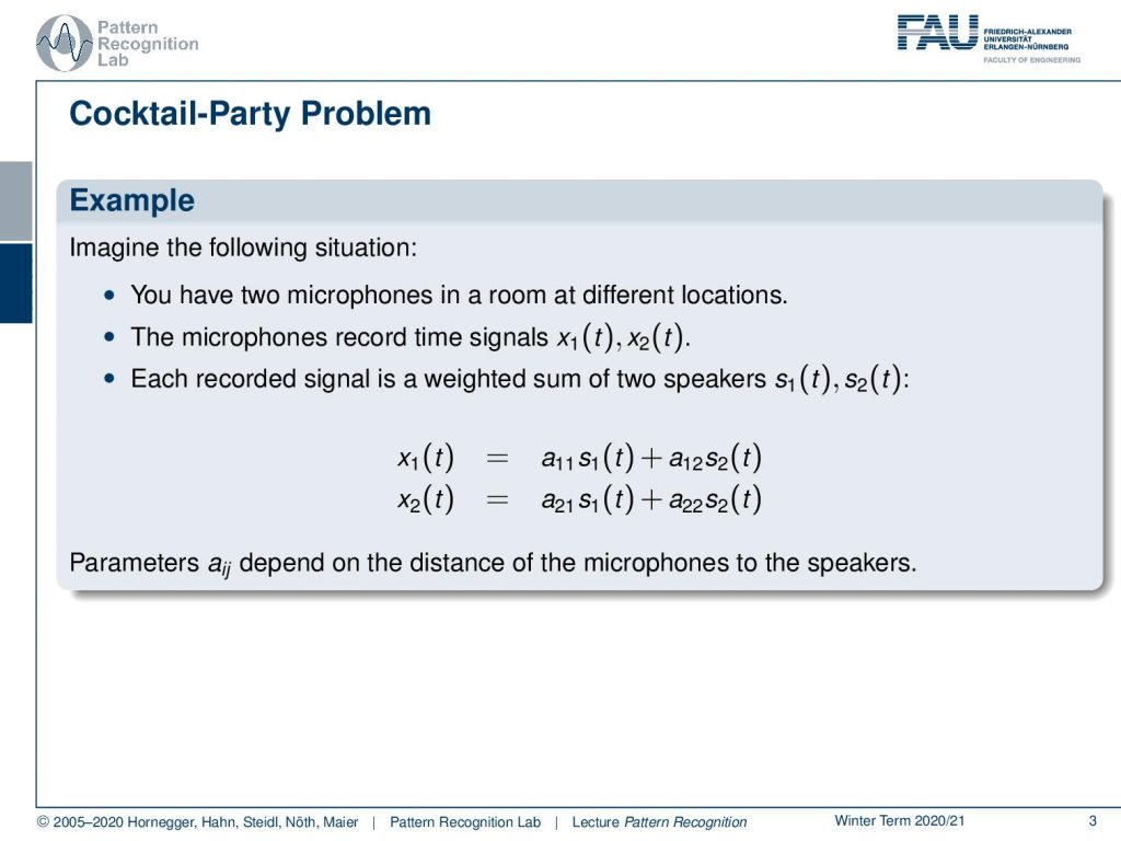
Let’s have a look at our slides. The Independent Component Analysis tries to address the cocktail party problem. Here imagine the situation that you have two microphones at different locations, and these microphones record some signal x₁ and x₂ that is dependent on the time. Now each recorded signal is essentially a weighted sum of the speakers in the room. For simplicity, let’s assume that there are two speakers in the room. We can model this essentially as a weighted sum of the two speakers that we collect in microphone one and microphone two. So the parameters depend essentially on the distance between the microphones and the speakers. Now we would be interested of course to reconstruct the signal from the two speakers. And this can be done using factorization methods and in particular the idea of the Independent Component Analysis.

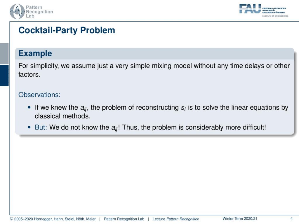
For simplicity, we just assume a very simple mixing model without any time delays or further factors here. This then means if we knew the a_ij, the problem of reconstructing s_i is to solve the linear equations by classical methods because we simply need to compute the inverse of this so-called mixing matrix. Now the problem is that we don’t know the a_ij. Thus, the problem is considerably more difficult and we can’t just use the matrix inverse of these unknown coefficients, so we have to estimate them as well.

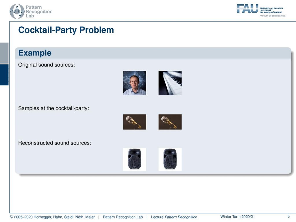
Now let’s look into a simple example. Here I brought two audio signals. One is me speaking, of course about machine learning. The other one is a piano that is playing some background music. Now you can see that what we would record at the microphone would then typically be a superposition of the two signals. So in one, you can hear that my voice is louder. In the other one, my voice is not as loud. Now the idea is that we want to find the unmixing matrix, and with the unmixing matrix, we can reconstruct the original audio signals. You can see this is a pretty hard task, but still, the results are quite impressive. Here you can hear my reconstructed voice from the superposition of the two signals and here you can hear the reconstructed music.

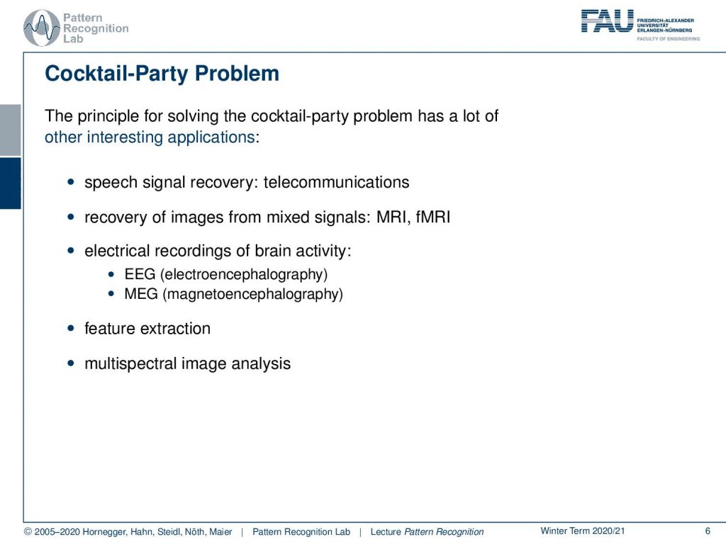
Generally, the cocktail party problem has many many more applications. It’s not just for unmixing two speakers or a sound source in the speaker. Generally, you can recover speech signals from telecommunications, you can recover images from mixed signals like an MRI and functional MRI. Then there are also examples where you can essentially reconstruct electrical recordings of the brain activity, so this is used in EEG and MEG signals. And of course, it is a popular way of extracting features, and you can even do multi-spectral image analysis with this.

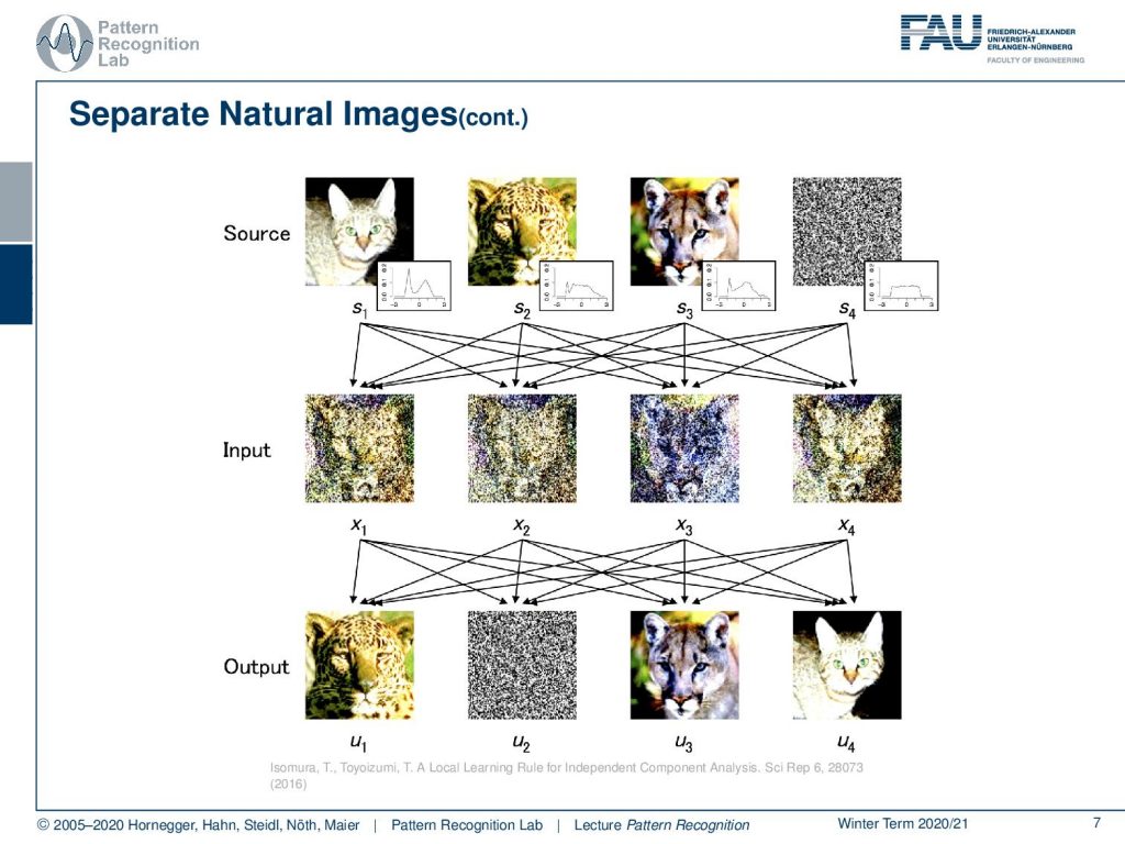
Let’s look into the separation of a natural image. Here you see that we have four different sources. So, it does not just work with two sources, but you can also just increase the size of the mixing matrix. Let’s look at a total of four sources. Then you mix them somehow with the input to our independent component analysis. You can see that essentially, we are close to not be able to recognize anything on those pictures. And then we perform the independent component analysis. You can see that it is very well reconstructed. We see that the different animals can be reconstructed and we also get a reconstruction of the noise. So generally, this is a method that has a broad range of applications. Note that the sequence of the images has changed. So this is a general drawback of the independent component analysis. We don’t get a ranking of the inputs, so we still have to look at the outputs and then identify which source has been mapped onto which output channel.

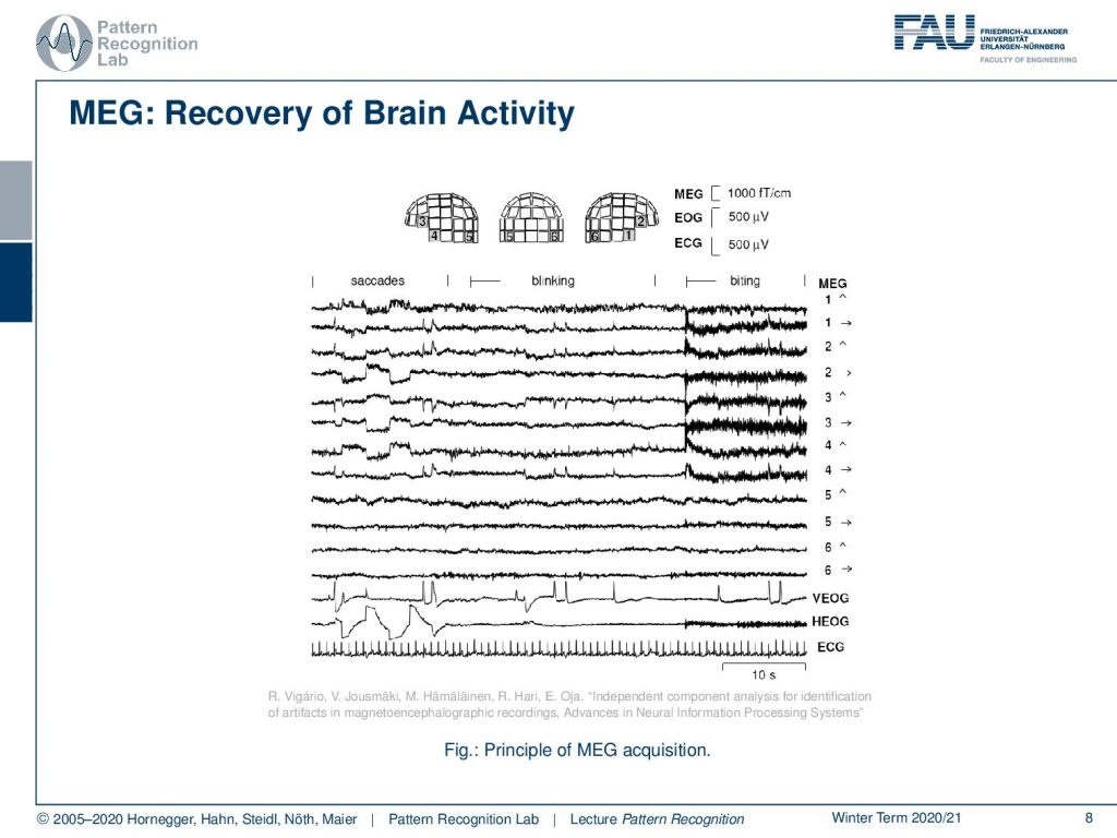
Now, this was an application in imaging. We can also use this to analyze brain activity. And here we are looking into a MEG acquisition. You see that the energy field is acquiring a superposition of all the different things that are happening in the brain. So we have a mixed signal that we are observing.

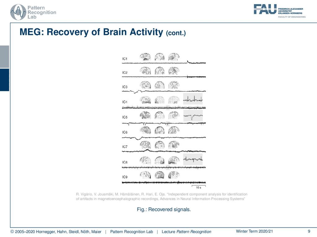
If we now apply an Independent Component Analysis, then we can reconstruct different activities in the brain. So we can use this method to localize different independent components and regions of activity in the brain.

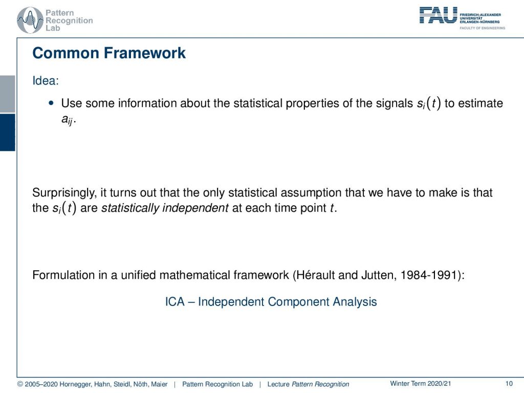
The common framework is that we have some information about the statistical properties of the signals to estimate the mixing coefficients a_ij. Now it turns out that the only statistical assumption that we have to make is that the signals are statistically independent at each time point t. This then gives rise to the independent component analysis that has been formulated in a unified mathematical framework by Hérault and Jutten in the years 1984 to 1991.

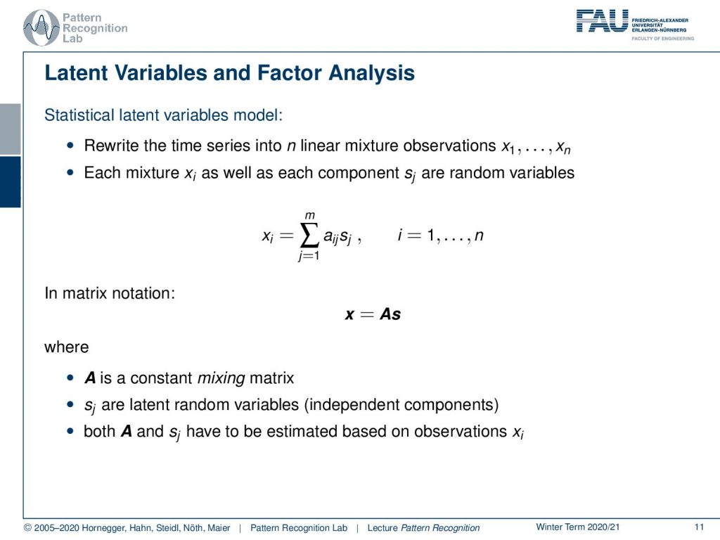
The idea is that we model this as statistical latent variables, and we rewrite the time series into n linear mixture observations. Then each mixture x_i, as well as each component s_j are random variables. So we have essentially the x_i that is computed as a superposition of the signals linearly. Now we can also write this in matrix notation. Then this would simply be x=As. And now A is a constant mixing matrix, so this doesn’t change. Then we have the latent random variables s_j, these are the independent components. Both A and s_j have to be estimated based on the observations x_i. Now, this is a pretty hard problem because we somehow need to factorize our signals. And you will see in the following that this problem is not unique.

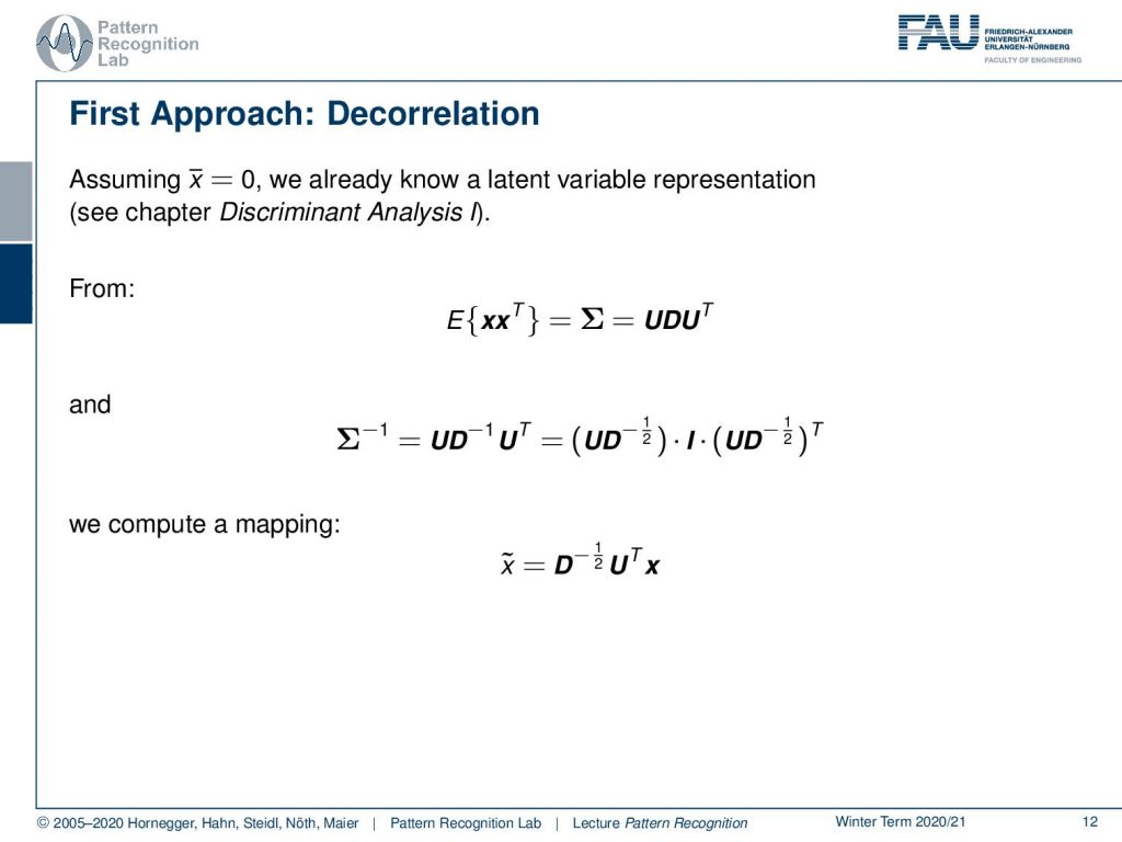
Let’s assume that we have a zero mean as we already did in the discriminant analysis. Then we can see that if we had a zero mean then we can express the expected value of xx^T, meaning the covariance matrix as UDU^T where this is the singular value decomposition of the covariance matrix. Now D is a diagonal matrix and U is an orthonormal matrix, which is essentially a rotation in this high dimensional space. We’ve also seen that if we compute the inverse, then we can essentially express this as 2 times this vector UD^-0.5 times the identity matrix, times the vector again transposed. So we can compute a mapping to a normalized space using exactly this feature transform.

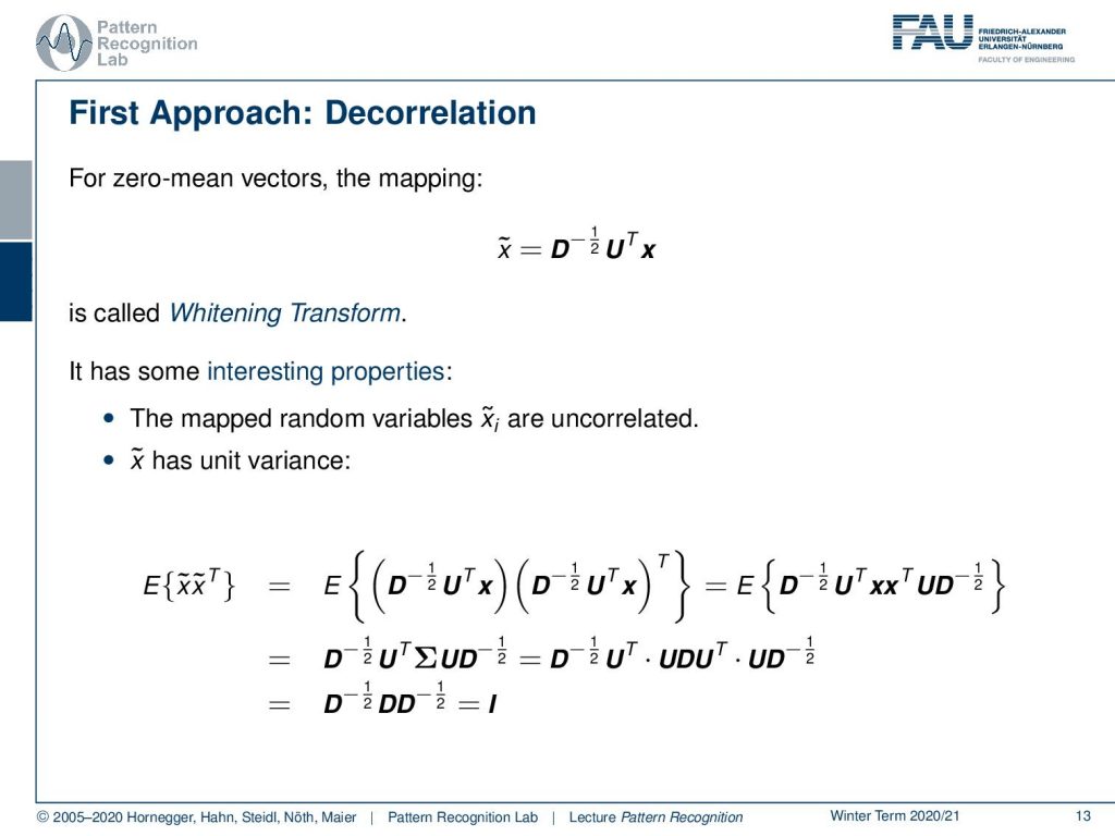
Now actually if we have zero mean vectors, this mapping is also known as the whitening transform because we essentially map everything onto a white noise. This has of course interesting properties. The mapped random variables x ̃_i are uncorrelated and x ̃ also has unit variance as you can see here. If I plug in x ̃, you get this feature transformed vectors. Then you can map it in this way. So you can see that the outer product of x and x^T can be rewritten as the covariance matrix of x. Then we can replace the factorization of the covariance matrix here. And then you see that essentially, all of this cancels out and in the very end, only the identity matrix remains.

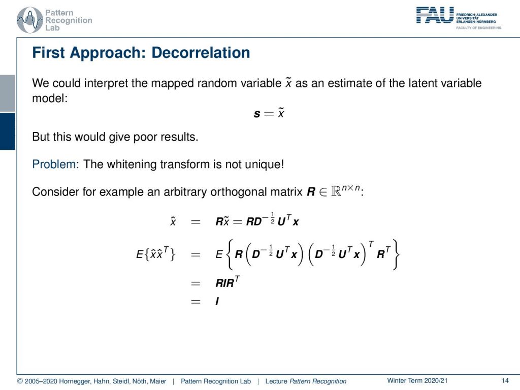
Let’s think about the first approach. We could interpret the mapped random variable x ̃ as an estimate of the latent variable model. And this would essentially then give us simply x ̃ as the solution to the signals but unfortunately, this gives us poor results. And the main problem is that this whitening transform is not unique. Now I can consider an arbitrary orthogonal matrix R and simply transform our x ̃ into some x ̂, and we simply add this matrix to the feature transform. If you look at this closely, then you can see that I can essentially apply the same trick for the expected value of x ̂. So we do the expected value of x ̂ times x ̂^T and this gives us again a kind of covariance matrix. We apply the same transformation as previously. We see that the inner part we already know cancels out to the identity matrix. And then we have R times the identity matrix times R^T. This is nothing else than the identity matrix. You can see we can choose an arbitrary orthogonal matrix R and multiply it to our whitening transform, and the property of being distributed with an identity matrix as a covariance matrix would not vanish. So there is essentially an infinite number of whitening transforms that all fulfill this property. So whitening is not just enough.

Next time in Pattern Recognition we want to look at the actual idea to construct the Independent Component Analysis, and we will see what additional steps are required to perform the unmixing of the signals. I hope you enjoyed the small video and you are all now very excited about Independent Component Analysis. We’ll see how to actually compute it in the next video. Thank you very much for watching and bye-bye! 

If you liked this post, you can find more essays here, more educational material on Machine Learning here, or have a look at our Deep Learning Lecture. I would also appreciate a follow on YouTube, Twitter, Facebook, or LinkedIn in case you want to be informed about more essays, videos, and research in the future. This article is released under the Creative Commons 4.0 Attribution License and can be reprinted and modified if referenced. If you are interested in generating transcripts from video lectures try AutoBlog.

References

1. A. Hyvärinen, E. Oja: Independent Component Analysis: Algorithms and Applications, Neural Networks, 13(4-5):411-430, 2000.
2. T. Hastie, R. Tibshirani, J. Friedman: The Elements of Statistical Learning, 2nd Edition, Springer, 2009.
3. T. M. Cover, J. A. Thomas: Elements of Information Theory, 2nd Edition, John Wiley & Sons, 2006.

Category: Lecture Notes in Pattern Recognition