Lecture Notes in Pattern Recognition: Episode 31 – EM Algorithm Example

These are the lecture notes for FAU’s YouTube Lecture “Pattern Recognition“. This is a full transcript of the lecture video & matching slides. We hope, you enjoy this as much as the videos. Of course, this transcript was created with deep learning techniques largely automatically and only minor manual modifications were performed. Try it yourself! If you spot mistakes, please let us know!

Welcome back to pattern recognition. Today we want to talk a bit about applications of the EM algorithm and I want to show one example from medical imaging where you can see how sophisticated those algorithms can get. I think that it will be very interesting for you to see how many additional steps we can actually model with this EM algorithm.

So let’s have a look at the slides that I have for you. So this is adaptive segmentation of MRI data and note that what I’m showing to you today is something that is let’s say an application. But it also involves many steps. So I would say topics like this one are very good for your understanding of how to bring these things into practice. But I don’t think that this algorithm presented in this video will be too relevant for the exam. So this is an application on MRI. So MRI is magnetic resonance imaging. It’s an important medical image acquisition technique. It has a high spatial resolution, good soft-tissue contrast, and does not involve any ionizing radiation. Several applications require segmentation. So here we do a voxel-wise classification where this voxel belongs into a certain tissue class and then you essentially assign every point in the image a class to which it belongs. These are typically tissue types. 

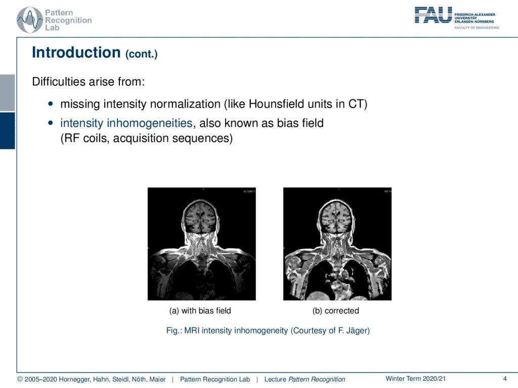
Now a problem arises in MRI that the intensities are not normalized. They’re not standardized in CT you would have things like the Hounsfield unit that would allow really a relation to a physical quantity. An MRI is very difficult and in many acquisition sequences, it is simply not standardized to a physical quantity. This then gives rise to intensity inhomogeneities that are also known as the bias field and this is introduced by the radiofrequency coils and the acquisition sequences. What then happens is that you get images like this one. So you acquire the image on the left-hand side which is now showing essentially the head and the upper part of the torso and you would assume that in a standardized image all the tissues would essentially have very similar gray values. But you can see that there is this kind of off-rolling effect that you see towards the boundaries of the image and you have a better contrast in the center than on the sides. But you can correct this with so-called bias field reduction algorithms like the one you have to see here on the right-hand side. By the way, this is work by the colleague Florian Jaeger who has actually written his PhD thesis about this topic. So now why is the bias field a problem?

Well, let’s say you have this checkerboard pattern here and you introduce a bias field. Then you can see that the checkerboard is still there so because human perception can compensate for those effects very efficiently. If you show an image like this one to let’s say your medical doctor he will say okay I can clearly see the checkerboard pattern. Now the bias field is multiplied here into this image. You can see that it introduces a change in the gray values and if you try to segment just using the gray value as a kind of tissue class or here indicating which part of the checkerboard you’re in, then you get segmentation results like this one. So you see that the actual gray value is not corresponding to the correct part of the checkerboard. Now of course this is also something that we typically then also have a couple of discussion with our medical partners because they say look I can see the checkerboard pattern why is your computer so stupid that it produces a result like this and you know every monkey can draw a pattern like the one that you see here on the right-hand side. So your computer is pretty stupid. 

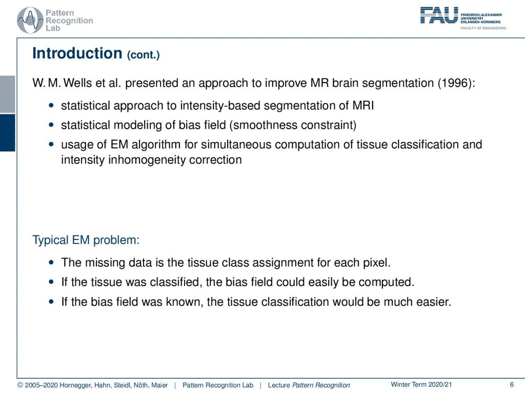
Now, of course, we have methods to deal with this and what I want to introduce here is actually going back to the work of Sandy Wells and he already presented the things that I’m showing in the lecture today in a paper in 1996. It is essentially a statistical approach to intensity-based segmentation of MRI. It is modeling the bias field also statistically using a smoothness constraint. Then he also used the EM algorithm for the simultaneous computation of the tissue classification and the intensity inhomogeneity correction. So the problem here is the missing data is the tissue class assignment for each pixel. We don’t know what is the actual class of the pixel and if the tissue were classified correctly then we could also very easily compute the bias field because we know it’s the deviation from the correct gray value to the one that we are observing. But if the bias field were known then also the tissue classification would be much easier. So again we have this kind of missing information problem here that in order to derive the tissue class from the gray value we need correct observations of the gray value. They are being hindered by the bias field. So we somehow have to simultaneously estimate both of them at the same time in order to solve the problem.

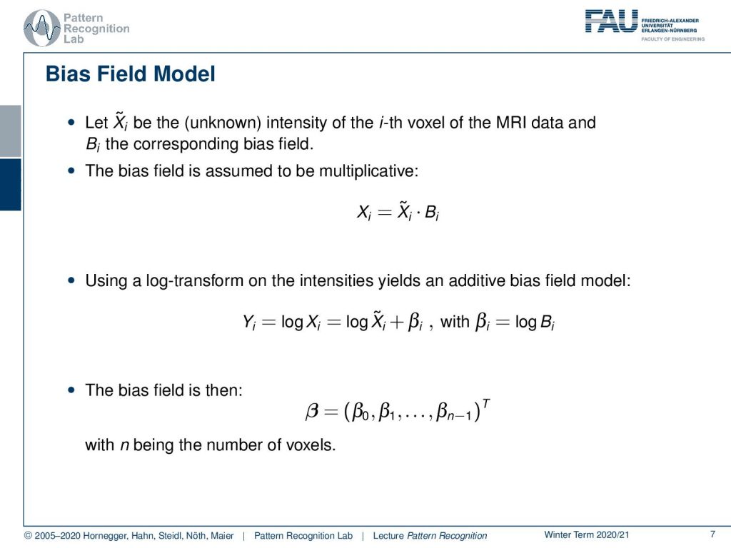
Now let’s have some X_i be the unknown intensity of the ith voxel of the MRI data and B the corresponding bias field. Then by physics, we know that the bias field in MRI is multiplicative which means the original intensity is multiplied with the bias. Now, this is a bit hard for our estimation. We don’t like to do this. So we can use the log transform in order to transform the intensities into an additive bias field. So we can apply the logarithm to our observations and then we see that we essentially convert the multiplication into an addition. Now we can describe the bias field now with β_i and the β_i is essentially the term for every pixel. Then we voxel if it’s a 3d volume and we essentially get one β for every voxel. 

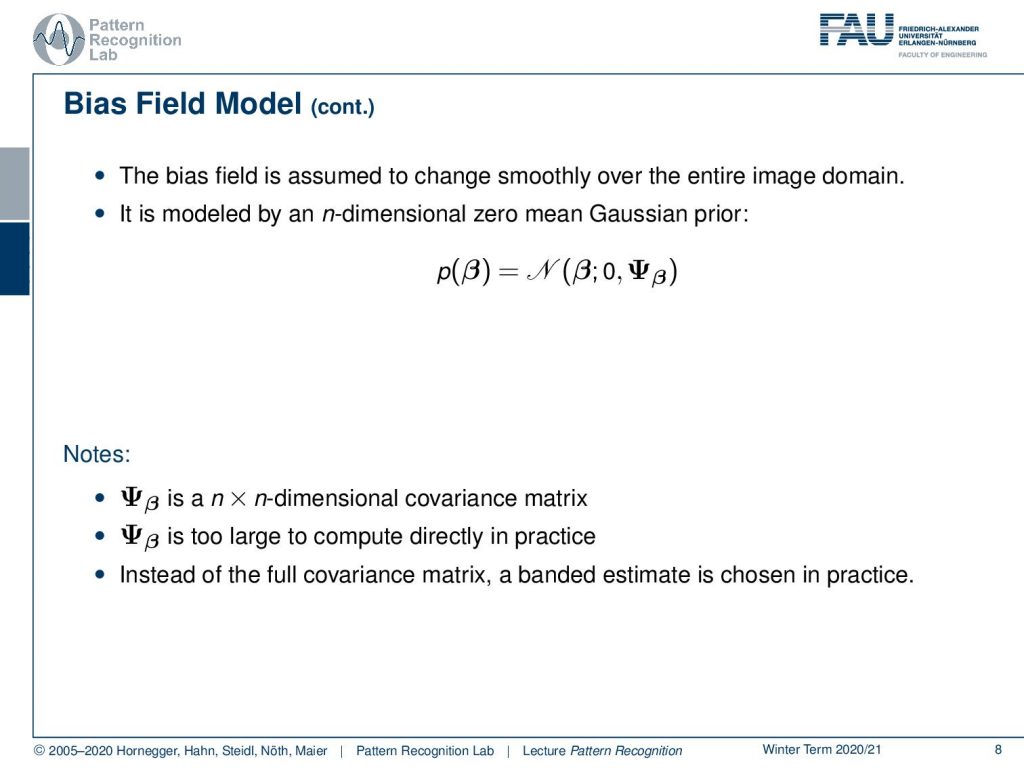
Now we assume that the bias field is changing smoothly over the entire image domain. This is modeled by an n-dimensional zero-mean Gaussian prior. So we assume that the intensities of our bias field are normally distributed. It has a zero mean and then there is a covariance matrix. This covariance matrix here is an n time n-dimensional matrix. Now, this is typically too large to be computed directly in practice. Note that we have the dimensionality of the image to the power of two. So this is a really large matrix. So what we do instead of the full covariance matrix, we put in a banded estimate to actually compensate for that. So this means essentially that we assume that a pixel is correlated only with neighboring pixels and far away distant pixels have no relation. This then allows us to describe the smoothness constraint.

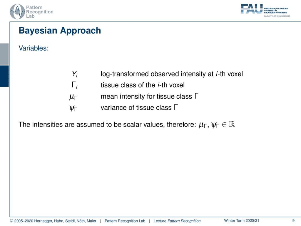
This brings us then to our list of variables so we have the Y_i which is the log-transformed observed intensity at the ith voxel so we observe that one then we have unknowns this is Γ_i which is the tissue class of the ith voxel. Then we have the μ_Γ which is the mean intensity for the tissue class in Γ and then we have some variance here for the tissue class of Γ. Now the intensities are assumed to be scalar values, therefore we see that the values here are the element of the real numbers. 

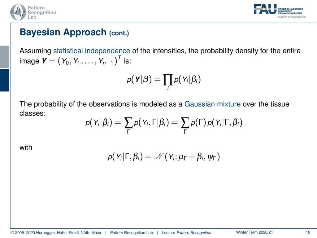
If we assume statistical independence of the intensities then the probability density for the entire image it can be written as a product. Now the probability of the observations is modeled as a Gaussian mixture over the tissue classes. So we have a sum over the individual probabilities for the observation and the class Γ given the bias field β_i and of course we can here marginalize over the class Γ and then we see that this is going to be the sum of the product of the prior of Γ with the respective component conditional probability. So here we choose to model our component dependent probability with a Gaussian and here then we have essentially the dependencies to μ_Γplus β_i and our respective variance. 

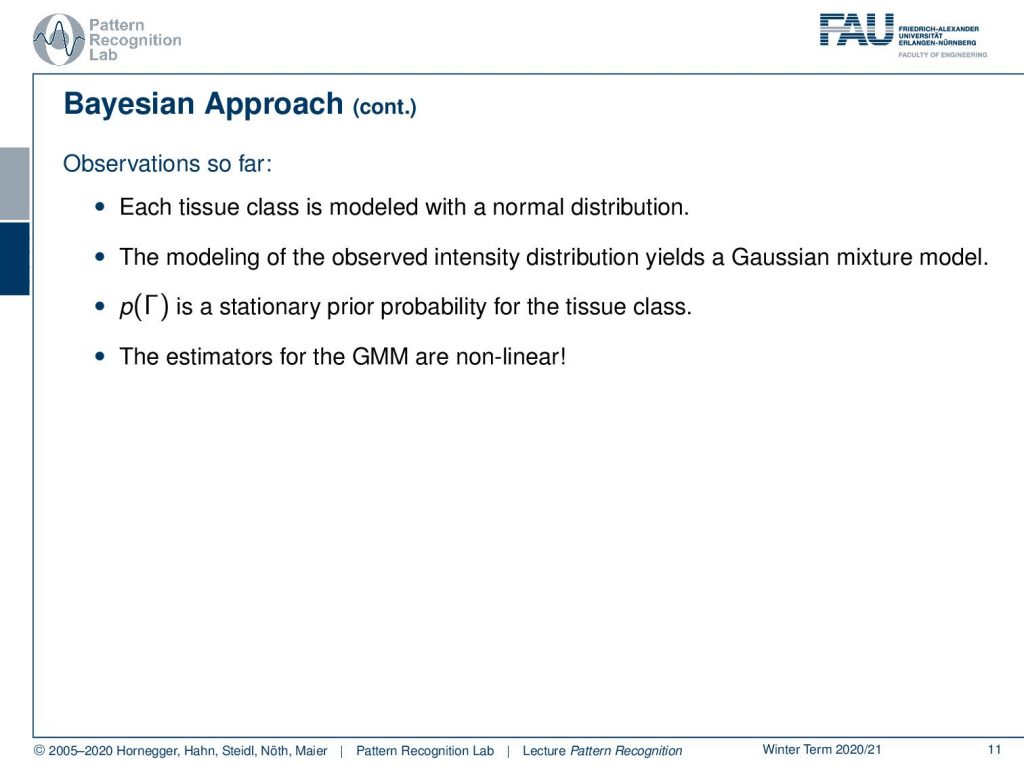
Now each tissue class is modeled with a normal distribution. The modeling of the observed intensity yields a Gaussian Mixture Model. The prior is a stationary prior for the tissue class. So if we have observations of similar anatomy they probably would produce a similar prior, because the tissue classes are distributed in a similar way. The estimators for the Gaussian Mixture Model are non-linear.

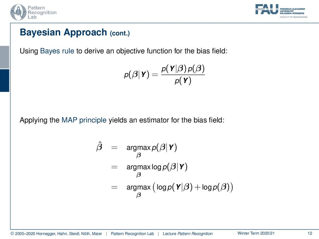
Let’s look into this issue a little more. So we will use a Bayesian approach here. So we use the Bayes rule to derive an objective function for the bias field. So the probability of the bias field given our observation is decomposed using the Bayes rule. Then we can essentially bring this into a Maximum a Posteriori estimator where we maximize the probability of β given y. This then can be transformed into a log-likelihood function just by applying the logarithm on our maximization. The next step then would be to apply the Bayes rule in the logarithm to apply Bayes rule in the logarithm and here you see that we already discarded the p(Y) because it’s irrelevant for our maximization. We simply end up with the logarithm of the conditional probability plus the logarithm of the prior of β. 

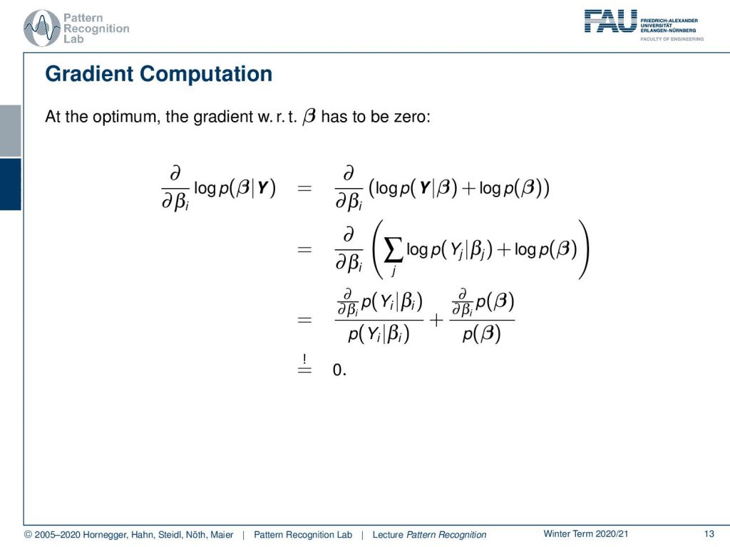
Now let’s look into this optimization a little bit more. So we have to compute the gradient with respect to β_i of the left-hand term and this is of course equivalent to the one on the right-hand side. So we can see now that we assumed that our probabilities are independent which means that we can write down the probability of Y given β as a product over the individual observations. If we use the logarithm we can convert this into a sum of logarithms and in the next step, we can compute the partial derivatives with respect to β_i. Here you see we use the property of the logarithm which means that we have to compute the partial derivative of p(Y_i) given β_i. Because we use the logarithm we have to divide by p(Y_i) given β_i and the same also holds true for the second term. So the logarithm disappears and we still have the partial derivatives in there. We need to set this to zero. 

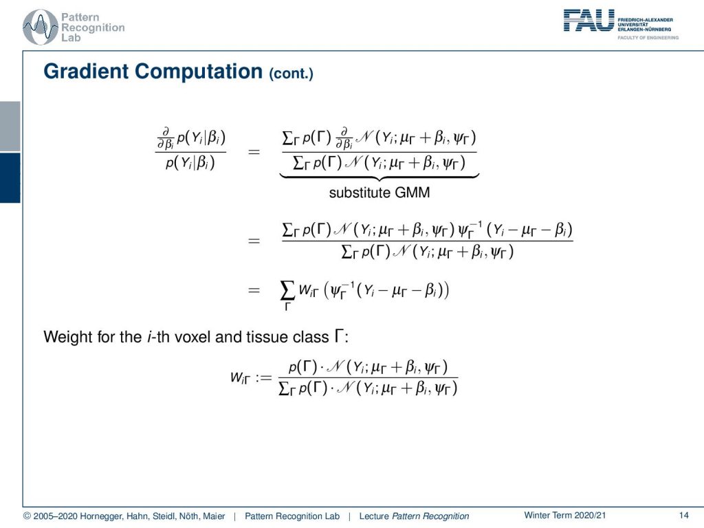
Now let’s plug in the definition of our Gaussian Mixture Model and we use the linearity here that we move the partial derivative with respect to β to the normal distribution. Then we still have to compute the partial derivative of the normal distribution with respect to β that then results in this additional multiplication with the inverse variance times Y_i minus μ_Γ minus β_i. Then we can further simplify this by introducing a weight W_iΓ and now W_iΓ is simply the prior times the normal distribution divided over the marginalization over the classes of the prior times the normal distribution.

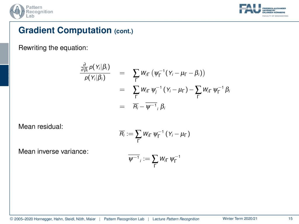
Now let’s look at this term in a little more detail. We can split this up into a part that is dependent on β and independent of β and this then allows us to write this as a mean residual minus a mean inverse variance times β_i. Now we can bring this back into our original formulation and now we switch to a matrix notation where we then have the mean residual as a matrix as well as this mean inverse covariance matrix here. We still have to finish up the gradient with respect to β according to our prior probability of β. Here we can see that this is then essentially the inverse covariance matrix of β and this has to be set to be zero. 

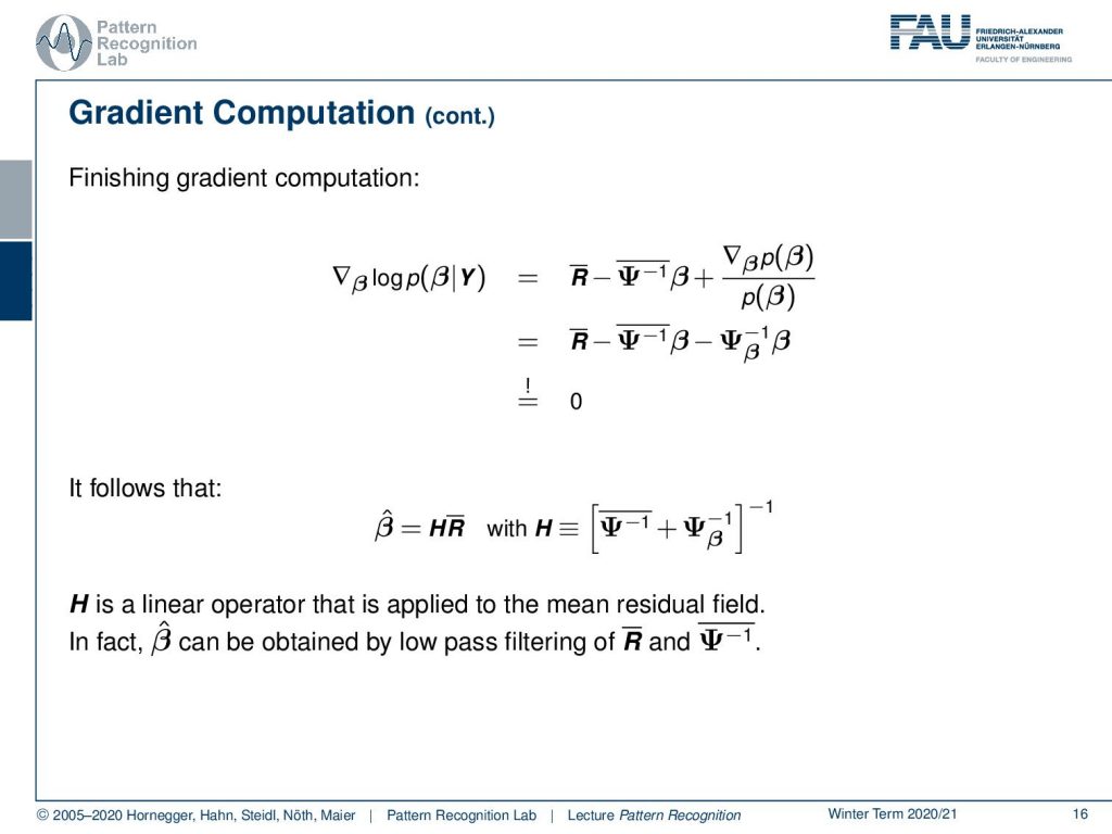
Now we can solve this for β̂ and β̂ can now be written as a simple matrix multiplication of H which is a new matrix that we are introducing here times the mean residual matrix. Now H is essentially the sum over the two inverted covariance terms and again inverted. So H is a linear operator that is applied to the mean residual field in fact β̂ can actually be obtained by low pass filtering of the mean residual and the mean inverse variances. 

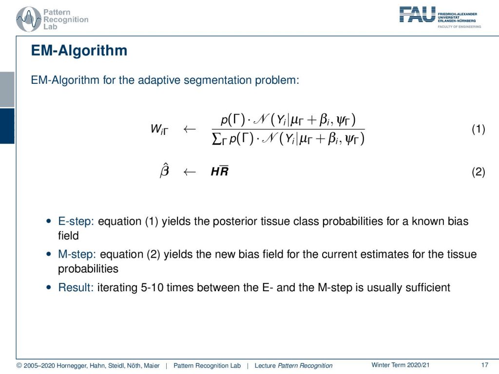
Now let’s write this up as an EM algorithm. The EM algorithm for the adaptive segmentation problem is now that we compute all of our W_iΓ which is essentially the E-step and then we estimate our new bias field which is the M-step. So equation one is the posterior tissue class probabilities for the known bias field. The M-step then estimates a new bias field for the current estimates of the tissue probabilities. So the result is generated iterating like five to ten times between the E and the M step and this is typically sufficient. I also have an example here which we got from Sandy Wells. 

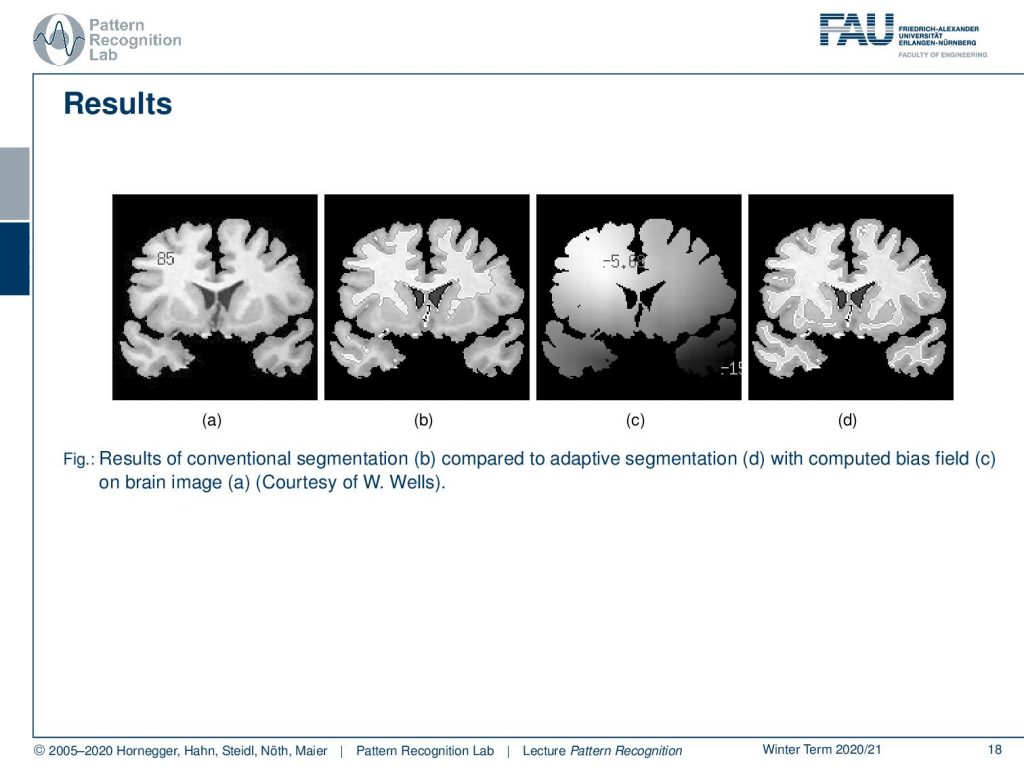
So we’re very happy that we can show this here. So on the left-hand side, you see the brain image in part b of this figure you see the initial segmentation which is pretty poor. Then we start estimating a bias field in c and with the correct bias field and also the segmentation is done much better than on the original image. 

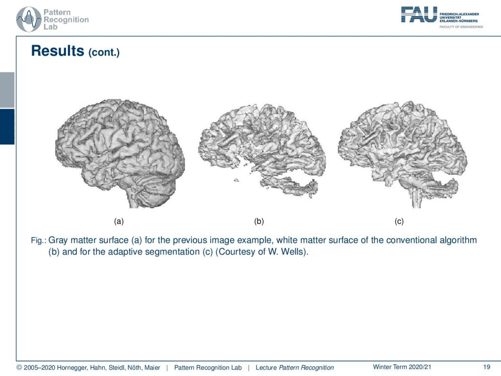
This can also be done in 3d. In 3d you can see much better how well the structure of the brain is preserved and how well you can actually do this adaptive segmentation.

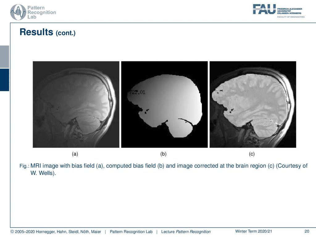
Now let’s look at some examples for bias fields. You can also correct the bias field and then produce a bias-corrected image and this is also a quite impressive visualization of what this algorithm can actually do. Note that we are only correcting for the brain tissue here and we didn’t correct for the surrounding tissues in this image. 

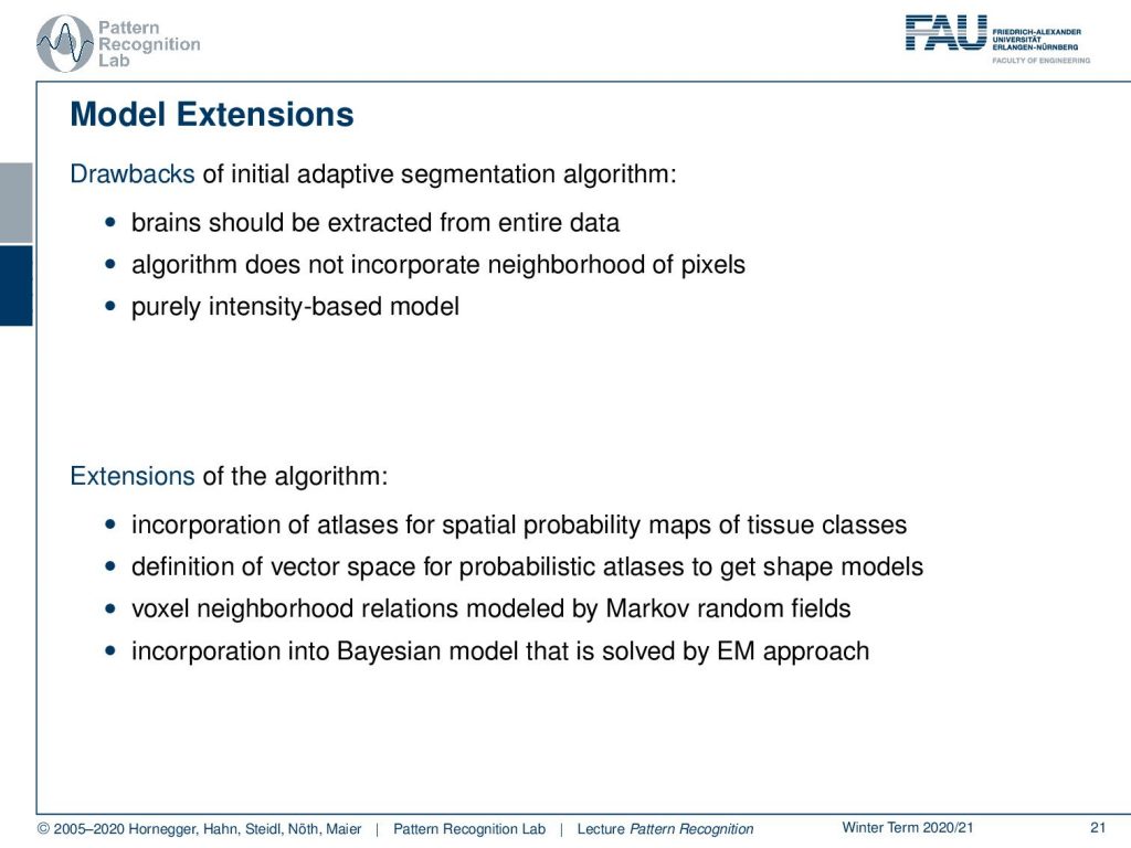
Well, there’s also a couple of drawbacks here. So the brains need to be extracted from the entire data. The algorithm does not really incorporate the neighborhood of pixels. It is a purely intensity-based model. Then we could essentially extend this by introducing atlases for the spatial probability maps of the tissue classes. You could define a vector space then for probabilistic atlases to get the shape model. Then you could have a voxel neighborhood relation that is modeled for example by Markov random fields. This actually can all be incorporated into a Bayesian model that is solved using an Expectation-Maximization type of approach.

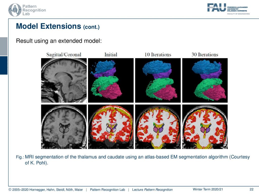
We have one example here that we can demonstrate from the work of K. Pohl and you see that you can get much better segmentations with such approaches. 

So what are the lessons learned? We have seen that the Bayesian approach can be also applied for MRI data segmentation. We can incorporate also bias field estimation as the hidden information that has to be extracted. We solve the non-linear problem iteratively using the EM algorithm. We’ve seen that we can also get further improvements by incorporating atlases of the anatomy. 

Now in the next lecture, we want to start talking about a new topic and this is going to be the Independent component analysis which is also a very powerful technique. I think it’s definitely a good idea to present it within our lecture. 

I do have some further readings for you. So there is the original paper by Sandy Wells, there is also a very good paper by Florian Jaeger on the non-rigid registration of joint histograms for intensity standardization in MRI and of course the works by K. Pohl where we were allowed to use some of the images.

So I also have some comprehensive questions for you that will help you in preparing for the exam and this brings us already to the end of this video. So I hope you enjoyed the small application that we looked into and looking forward to seeing you in the next video. Bye-bye!

If you liked this post, you can find more essays here, more educational material on Machine Learning here, or have a look at our Deep Learning Lecture. I would also appreciate a follow on YouTube, Twitter, Facebook, or LinkedIn in case you want to be informed about more essays, videos, and research in the future. This article is released under the Creative Commons 4.0 Attribution License and can be reprinted and modified if referenced. If you are interested in generating transcripts from video lectures try AutoBlog

References  

1. Original paper on adaptive MRI segmentation: W. M. Wells, R. Kikinis, W. E. L. Grimson, F. Jolesz: Adaptive segmentation of MRI data, IEEE Transactions on Medical Imaging, 15:429-442, 1996. 
2.  F. Jäger, J. Hornegger: Nonrigid registration of joint histograms for intensity standardization in magnetic resonance imaging, IEEE Transactions on Medical Imaging, 28(1):137-150, 2009.
3. K. M. Pohl, J. Fisher, J. J. Levitt, M. E. Shenton, R. Kikinis, W. E. L. Grimson, W. M. Wells: A Unifying Approach to Registration, Segmentation, and Intensity Correction, Proc. MICCAI, pp. 310-318, 2005. 
4.  K. M. Pohl, J. Fisher, S. Bouix, M. E. Shenton, R. W. McCarley, W. E. L. Grimson, R. Kikinis, W. M. Wells: Using the logarithm of odds to define a vector space on probabilistic atlases, Medical Image Analysis, 11(6), pp. 465-477, 2007.

Category: Lecture Notes in Pattern Recognition