
Contrastive Losses
These are the lecture notes for FAU’s YouTube Lecture “Deep Learning“. This is a full transcript of the lecture video & matching slides. We hope, you enjoy this as much as the videos. Of course, this transcript was created with deep learning techniques largely automatically and only minor manual modifications were performed. Try it yourself! If you spot mistakes, please let us know!
Welcome back to deep learning! So, today we want to discuss in the last part about weakly and self-supervised learning: a couple of new losses that can also help us with the self-supervision. So, let’s see what we have on our slides: Today part number four and the idea is contrastive self-supervised learning.
In contrastive learning, you try to formulate the learning problem as a kind of matching approach. So here, we have an example from supervised learning. The idea is then to match the correct animal with respect to other animals. The learning task is whether the animal is the same or a different one. This is actually a very powerful form of training because you can avoid a couple of disadvantages in generative or context models. For example, pixel-level losses could overly focus on pixel-based details and pixel-based objectives often assume pixel independence. This reduces the ability to model correlations or complex structures. Here, we essentially can then build abstract models that are also built in a kind of hierarchical way. Now, we have this supervised example but of course, this also works with many of the different pseudo-labels that we’ve seen earlier.
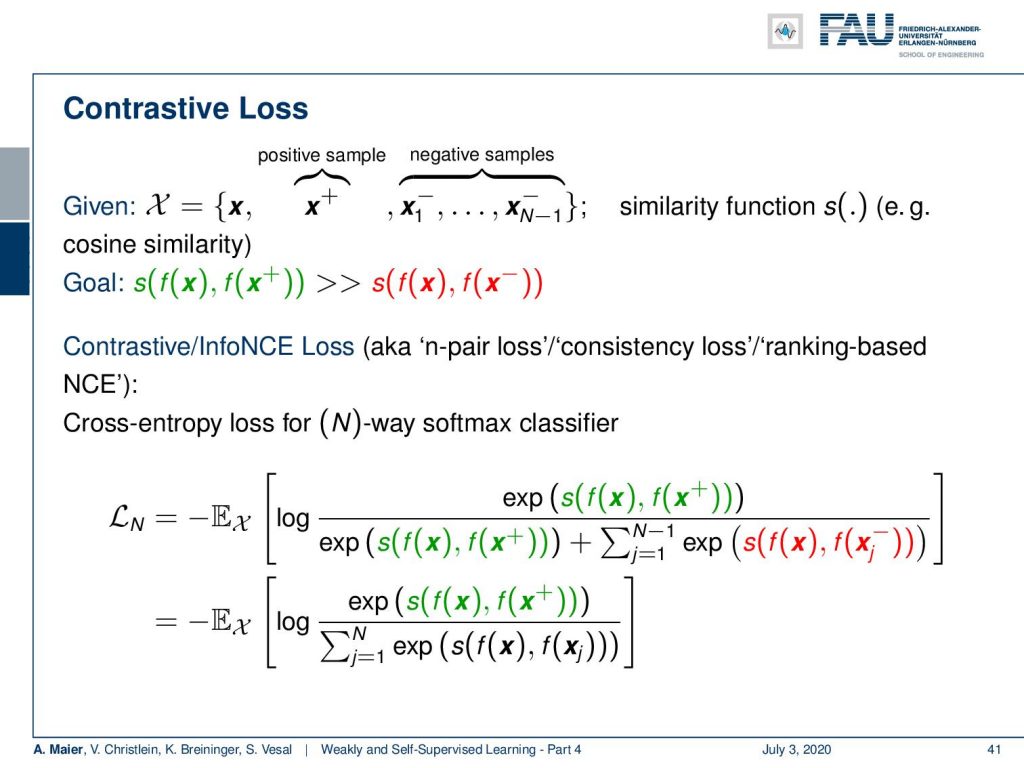
We can then build this contrastive loss. All that we need is the current sample x some positive sample x plus and then negative samples that are all from a different class. In addition, we need a similarity function s and this could, for example, be a cosine similarity. You could also have a trainable similarity function but generally, you can also use some of the standard similarity functions that we already discussed in this lecture. Furthermore, you want to apply then your network f(x) and compute the similarity. The goal is then to have a higher similarity between the positive sample and the sample under consideration and all the negative ones. This then leads to the contrastive loss. It’s sometimes also called the info normalized cross-entropy loss. There are also other names in literature: The n-pair loss, consistency loss, and the ranking based NCE. It’s essentially a cross-entropy loss for an n-way softmax classifier. The idea here is that you then have essentially the positive examples and this is then normalized by all of the examples. Here, I’m splitting the two still in the first row, but you can then simply see that the split is actually a sum over all of the samples. This then yields a kind of softmax classifier.
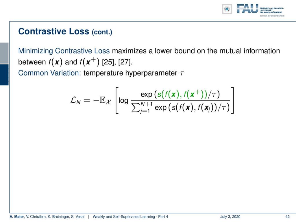
So minimizing the contrastive loss actually maximizes a lower bound on the mutual information between f(x) and f(x plus) as shown in those two references here. There is also a common variation that introduces a temperature hyperparameter that is shown in this example. So, you divide by an additional τ.
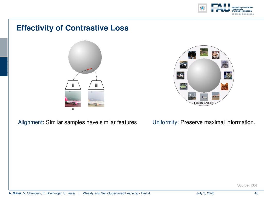
The contrastive losses are very effective and they have two very useful properties. On the one hand, they align. So, similar samples have similar features. On the other hand, they create uniformity because they preserve the maximal information.
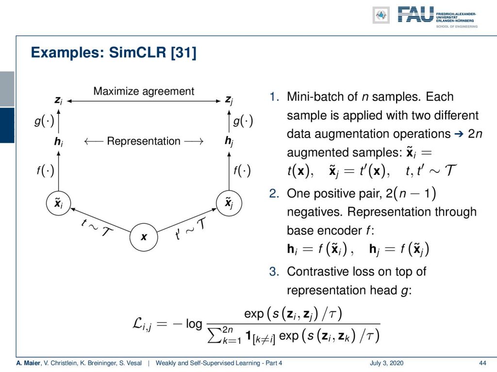
Let’s look into an example of how this can be constructed. This is from [31]. Here, you can see that we can for example start with some sample x. So let’s say you start with a mini-batch of n samples. Then, each sample is transformed with two different data augmentation operations. This leads to 2n augmented samples. So for every sample in the batch, you get two different augmentations. Here, we take t and t’ that we apply to the same sample. This sample is then the same and your transformations t and t’ are taken from a set of augmentations T. Now, you end up with one positive pair for each sample and 2(n-1) negative pairs. Because they’re all different samples, you are able to compute a representation through the base encoder f(x) that then produces some h which is the actual feature representation that we’re interested in. An example of f(x) could be a ResNet-50. On top of this, we have a representation head g that then does an additional dimensionality reduction. Note that both g and f are the same in both branches. So, you could argue this approach has considerable similarities to what is called a Siamese network. So, you then obtain two different sets z subscript i and z subscript j from g. With those z, you can compute your contrastive loss that is then expressed as the similarity between the two z over the temperature parameter τ. You see, this is essentially the same contrastive loss that we have already seen earlier.
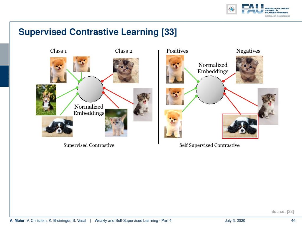
Contrastive losses, of course, can also be combined in a supervised way. This then leads to supervised contrastive learning. Here, the idea is that if you just perform the self-supervised contrastive, you have positive examples versus the negative ones. With the supervised contrastive loss, you can then also embed additional class information.
So, this has additional positive effects. Let’s see how this is applied. We remain essentially with the same idea of training two coupled networks.
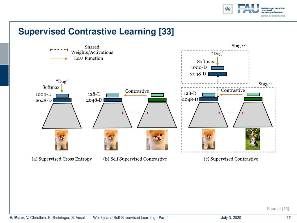
So let’s summarize a bit of what the difference between contrastive learning and supervised contrastive learning is. Well, in supervised learning, you would essentially have your encoder that is shown here as this gray block. Then, you end up with some description that is a 2048 dimensional vector and you further train a classification head that produces the class dog using the classical cross-entropy loss. Now, in contrastive learning, you would then expand on this. You would have essentially two coupled networks and you have two patches that are either the same or not the same with a different augmentation technique. You train these coupled weight-shared networks to produce 2048 dimensional representations. On top, you have this representation head and you use the contrastive loss on the representation layer itself. Now, if you combine the two supervised and contrastive, you essentially have the same setup as in the contrastive loss, but on the representation layer, you can then augment with an additional loss that works strictly supervised. There, you still have the typical softmax that goes to let’s say a thousand classes and predicts dog in this example. You couple it on the representation layer to be able to fuse contrastive and supervised losses.
So, the self-supervised has no knowledge about the class labels and it only knows about one positive example. The supervised has knowledge about all the class labels and has many positives per example. This then can be combined and you compute the loss between any sample z having the same class anchor. This then allows you to compute a loss between any sample z subscript j having the same class as the anchor z subscript i. So, the two classes are the same. This leads to the following loss: You can see this is still based on this kind of contrastive loss. Now, we explicitly use the cosine similarity just using the inner product of the two vectors. Also, you can see that we essentially add the red terms here that tell us to only use cases where we have different samples. So i is unequal to j and we want to use samples in this loss where we want to use samples in this loss, where the actual class membership is the same.
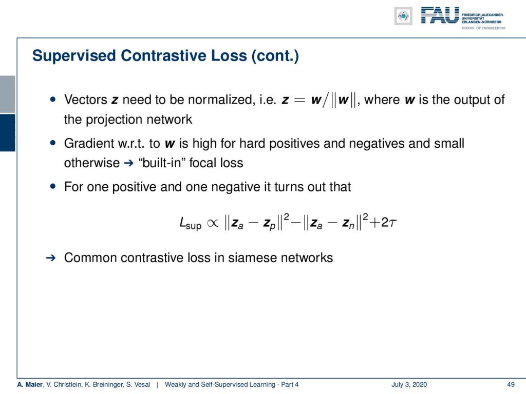
There are a couple of additional things that you have to keep in mind. The vectors z need to be normalized. This means that you want to introduce a scaling where this w is essentially the output of the projection network and you scale it such that it has a unit norm. This then essentially leads to something that you could interpret as a built-in focal loss because the gradient with respect to w is going to be high for hard positives and negatives and small otherwise. So, for one positive and one negative, by the way, it turns out that this loss is proportional to the Euclidean distance squared between the actual observation and the positive minus the Euclidean distance squared between the actual observation and the negative. This is, by the way, also a very common contrastive loss in Siamese networks.
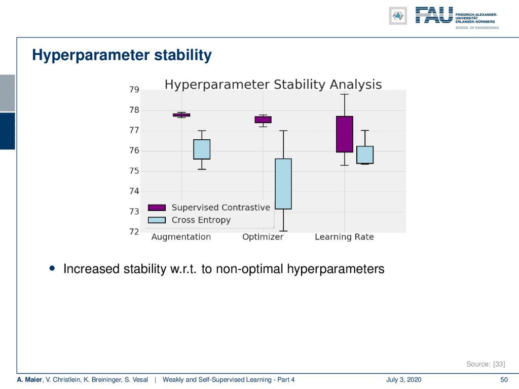
Let’s have a look at the hyperparameters. It turns out that the supervised contrastive loss is also very stable with respect to hyperparameters and you don’t see these large variations as if you were using only supervised cross-entropy loss in terms of the learning rate, in terms of the optimizer, as well as in terms of the augmentation. If you’re interested in the exact experimental details please have a look at [33].
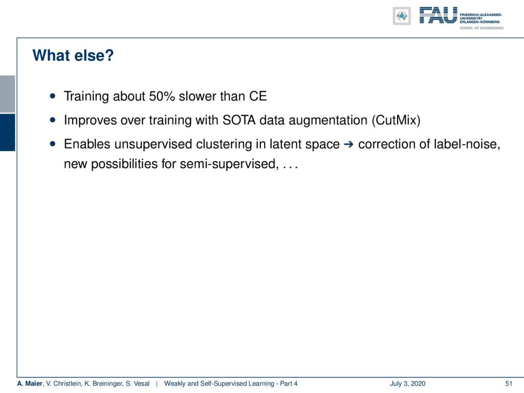
What else? Well, the training is about 50% slower than with the cross-entropy loss. It does improve over training with state-of-the-art data augmentation like CutMix and it enables unsupervised clustering in latent space. This allows them to correct for label noise. It also introduces new possibilities for semi-supervised learning and so on.
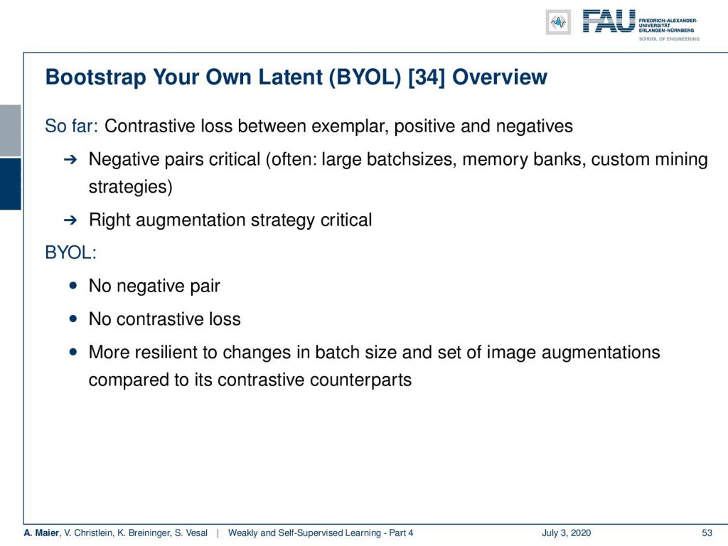
Well, is that it? Are there no more ideas? Well, there’s also some interesting idea that is bootstrapping self-supervised learning. You could argue that this is a paradigm change. This is a very new paper, but I’m including it here because it has some very interesting ideas that are very different from the contrastive losses. So it’s called bootstrap your own latent (BYOL) and the problem that they observe is that the choice of pairs is critical. So, often you need to have large batch sizes, memory banks, and custom mining strategies in order to get those pairs right. You also need to have the right augmentation strategy. In bootstrap your own latent, they don’t need negative pairs. they don’t need contrastive loss, and they’re more resilient to changes in batch size and the set of image augmentations compared to contrastive counterparts.
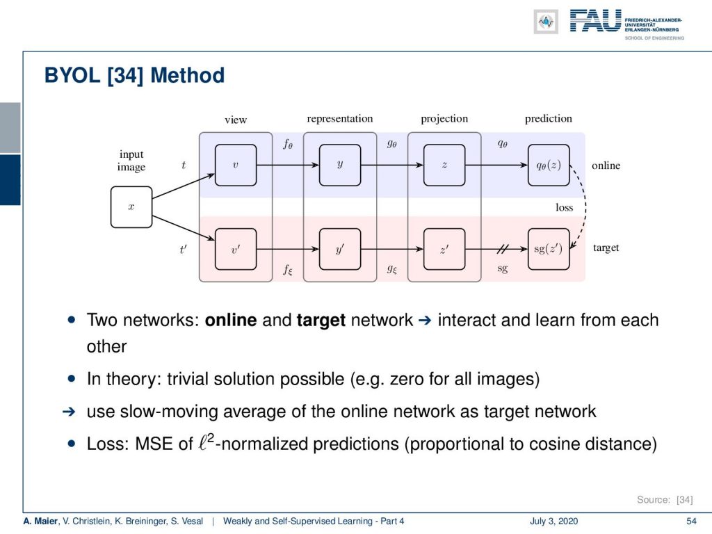
What’s the idea? Well, they have a similar setup here. They have this kind of network that does the view, representation, projection, and prediction. Now, the idea is that they have an online and a target network. They interact and learn from each other. Now, of course, this is problematic because in theory there’s a trivial solution possible like zero for all images. So, what they then use to counter that is they use a slow-moving average of the online network as the target network. This prevents from collapsing or weights to zero very quickly. As loss they use the mean square error of the l2 normalized predictions. This is proportional to the cosine distance.
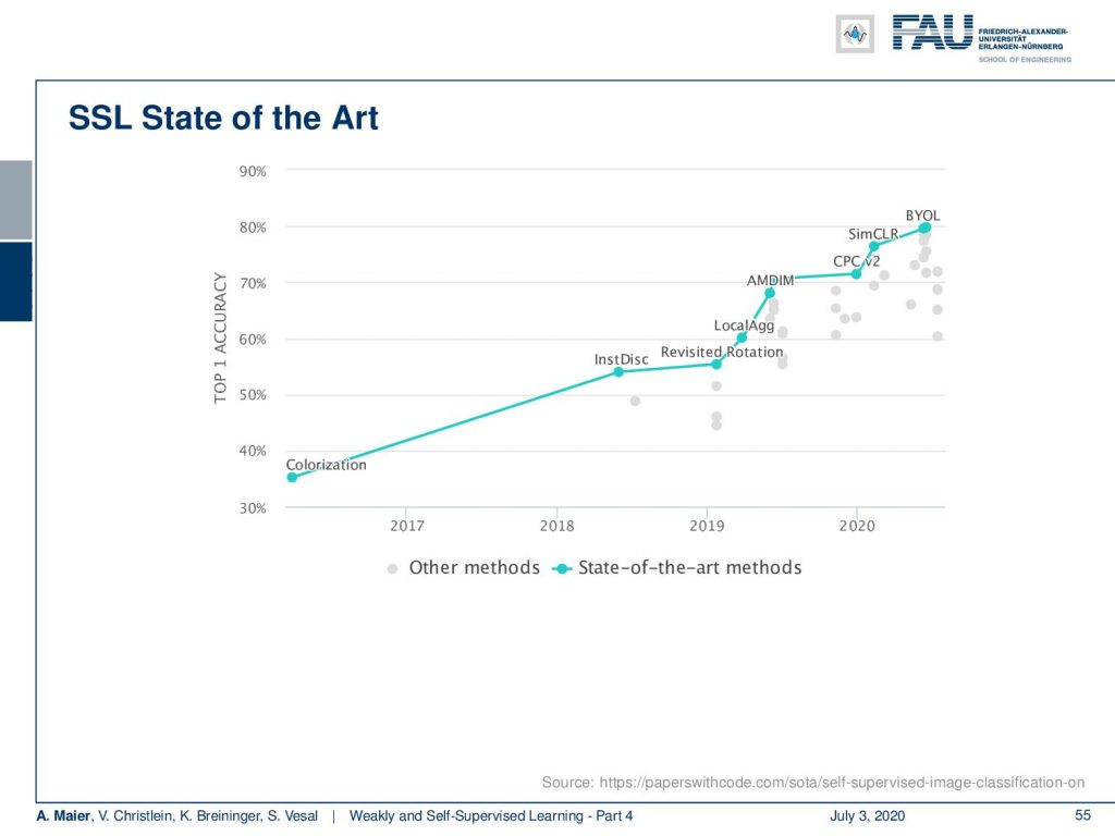
It’s quite interesting that with this very simple idea, they actually outperform the state-of-the-art and self-supervised learning approaches. So, you can see here colorization and different ideas that we talked about in the beginning and simCLR. They outperform them with their approach. They outperform even simCLR.
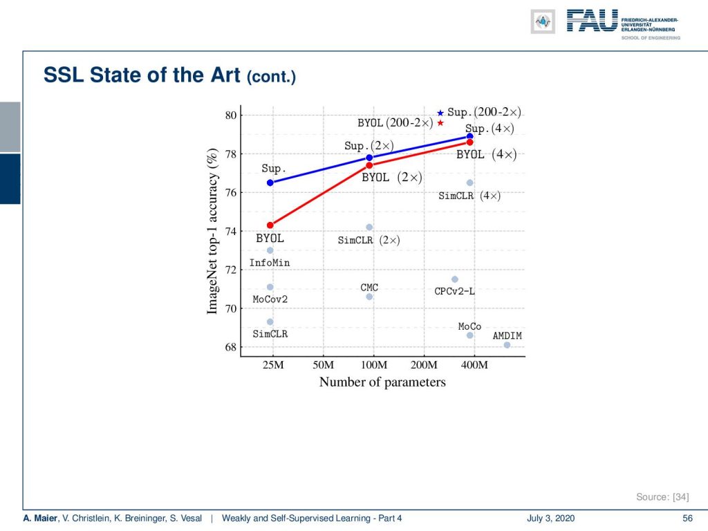
It’s quite interesting to see that also in terms of the number of parameters they are very close to supervised learning with respect to top-1 image accuracy on ImageNet. So, they get very close to state-of-the-art performance with very simple approaches. Actually I’m quite interested in seeing whether this will also be transferable to other domains than ImageNet. In particular, it would be interesting to look into such approaches on medical data, for example. You see that with the self-supervised learning we’re very very close to the state-of-the-art. This is a very active field of research. So, let’s see how these results will develop in the next couple of months and years and which of the approaches will be considered state-of-the-art methods in a couple of months from now.
Of course, we are now slowly going towards the end of our lecture. But there are still some things coming up next time. In particular, next time we want to talk about how to process graphs. So there’s also something which is a very nice concept called graph convolutions and I want to introduce you to this topic in one of the next videos. Another emerging method that I still want to show is an idea of how to avoid learning everything from scratch and how to embed specific prior knowledge into deep networks. There are also some very cool approaches out there that I think deserve being presented in this lecture. So, I have plenty of references below. So, thank you very much for listening and looking forward to seeing you in the next video. Bye-bye!
If you liked this post, you can find more essays here, more educational material on Machine Learning here, or have a look at our Deep LearningLecture. I would also appreciate a follow on YouTube, Twitter, Facebook, or LinkedIn in case you want to be informed about more essays, videos, and research in the future. This article is released under the Creative Commons 4.0 Attribution License and can be reprinted and modified if referenced. If you are interested in generating transcripts from video lectures try AutoBlog.
References
[1] Özgün Çiçek, Ahmed Abdulkadir, Soeren S Lienkamp, et al. “3d u-net: learning dense volumetric segmentation from sparse annotation”. In: MICCAI. Springer. 2016, pp. 424–432.
[2] Waleed Abdulla. Mask R-CNN for object detection and instance segmentation on Keras and TensorFlow. Accessed: 27.01.2020. 2017.
[3] Olga Russakovsky, Amy L. Bearman, Vittorio Ferrari, et al. “What’s the point: Semantic segmentation with point supervision”. In: CoRR abs/1506.02106 (2015). arXiv: 1506.02106.
[4] Marius Cordts, Mohamed Omran, Sebastian Ramos, et al. “The Cityscapes Dataset for Semantic Urban Scene Understanding”. In: CoRR abs/1604.01685 (2016). arXiv: 1604.01685.
[5] Richard O. Duda, Peter E. Hart, and David G. Stork. Pattern classification. 2nd ed. New York: Wiley-Interscience, Nov. 2000.
[6] Anna Khoreva, Rodrigo Benenson, Jan Hosang, et al. “Simple Does It: Weakly Supervised Instance and Semantic Segmentation”. In: arXiv preprint arXiv:1603.07485 (2016).
[7] Kaiming He, Georgia Gkioxari, Piotr Dollár, et al. “Mask R-CNN”. In: CoRR abs/1703.06870 (2017). arXiv: 1703.06870.
[8] Sangheum Hwang and Hyo-Eun Kim. “Self-Transfer Learning for Weakly Supervised Lesion Localization”. In: MICCAI. Springer. 2016, pp. 239–246.
[9] Maxime Oquab, Léon Bottou, Ivan Laptev, et al. “Is object localization for free? weakly-supervised learning with convolutional neural networks”. In: Proc. CVPR. 2015, pp. 685–694.
[10] Alexander Kolesnikov and Christoph H. Lampert. “Seed, Expand and Constrain: Three Principles for Weakly-Supervised Image Segmentation”. In: CoRR abs/1603.06098 (2016). arXiv: 1603.06098.
[11] Tsung-Yi Lin, Michael Maire, Serge J. Belongie, et al. “Microsoft COCO: Common Objects in Context”. In: CoRR abs/1405.0312 (2014). arXiv: 1405.0312.
[12] Ramprasaath R. Selvaraju, Abhishek Das, Ramakrishna Vedantam, et al. “Grad-CAM: Why did you say that? Visual Explanations from Deep Networks via Gradient-based Localization”. In: CoRR abs/1610.02391 (2016). arXiv: 1610.02391.
[13] K. Simonyan, A. Vedaldi, and A. Zisserman. “Deep Inside Convolutional Networks: Visualising Image Classification Models and Saliency Maps”. In: Proc. ICLR (workshop track). 2014.
[14] Bolei Zhou, Aditya Khosla, Agata Lapedriza, et al. “Learning deep features for discriminative localization”. In: Proc. CVPR. 2016, pp. 2921–2929.
[15] Longlong Jing and Yingli Tian. “Self-supervised Visual Feature Learning with Deep Neural Networks: A Survey”. In: arXiv e-prints, arXiv:1902.06162 (Feb. 2019). arXiv: 1902.06162 [cs.CV].
[16] D. Pathak, P. Krähenbühl, J. Donahue, et al. “Context Encoders: Feature Learning by Inpainting”. In: 2016 IEEE Conference on Computer Vision and Pattern Recognition (CVPR). 2016, pp. 2536–2544.
[17] C. Doersch, A. Gupta, and A. A. Efros. “Unsupervised Visual Representation Learning by Context Prediction”. In: 2015 IEEE International Conference on Computer Vision (ICCV). Dec. 2015, pp. 1422–1430.
[18] Mehdi Noroozi and Paolo Favaro. “Unsupervised Learning of Visual Representations by Solving Jigsaw Puzzles”. In: Computer Vision – ECCV 2016. Cham: Springer International Publishing, 2016, pp. 69–84.
[19] Spyros Gidaris, Praveer Singh, and Nikos Komodakis. “Unsupervised Representation Learning by Predicting Image Rotations”. In: International Conference on Learning Representations. 2018.
[20] Mathilde Caron, Piotr Bojanowski, Armand Joulin, et al. “Deep Clustering for Unsupervised Learning of Visual Features”. In: Computer Vision – ECCV 2018. Cham: Springer International Publishing, 2018, pp. 139–156. A.
[21] A. Dosovitskiy, P. Fischer, J. T. Springenberg, et al. “Discriminative Unsupervised Feature Learning with Exemplar Convolutional Neural Networks”. In: IEEE Transactions on Pattern Analysis and Machine Intelligence 38.9 (Sept. 2016), pp. 1734–1747.
[22] V. Christlein, M. Gropp, S. Fiel, et al. “Unsupervised Feature Learning for Writer Identification and Writer Retrieval”. In: 2017 14th IAPR International Conference on Document Analysis and Recognition Vol. 01. Nov. 2017, pp. 991–997.
[23] Z. Ren and Y. J. Lee. “Cross-Domain Self-Supervised Multi-task Feature Learning Using Synthetic Imagery”. In: 2018 IEEE/CVF Conference on Computer Vision and Pattern Recognition. June 2018, pp. 762–771.
[24] Asano YM., Rupprecht C., and Vedaldi A. “Self-labelling via simultaneous clustering and representation learning”. In: International Conference on Learning Representations. 2020.
[25] Ben Poole, Sherjil Ozair, Aaron Van Den Oord, et al. “On Variational Bounds of Mutual Information”. In: Proceedings of the 36th International Conference on Machine Learning. Vol. 97. Proceedings of Machine Learning Research. Long Beach, California, USA: PMLR, Sept. 2019, pp. 5171–5180.
[26] R Devon Hjelm, Alex Fedorov, Samuel Lavoie-Marchildon, et al. “Learning deep representations by mutual information estimation and maximization”. In: International Conference on Learning Representations. 2019.
[27] Aaron van den Oord, Yazhe Li, and Oriol Vinyals. “Representation Learning with Contrastive Predictive Coding”. In: arXiv e-prints, arXiv:1807.03748 (July 2018). arXiv: 1807.03748 [cs.LG].
[28] Philip Bachman, R Devon Hjelm, and William Buchwalter. “Learning Representations by Maximizing Mutual Information Across Views”. In: Advances in Neural Information Processing Systems 32. Curran Associates, Inc., 2019, pp. 15535–15545.
[29] Yonglong Tian, Dilip Krishnan, and Phillip Isola. “Contrastive Multiview Coding”. In: arXiv e-prints, arXiv:1906.05849 (June 2019), arXiv:1906.05849. arXiv: 1906.05849 [cs.CV].
[30] Kaiming He, Haoqi Fan, Yuxin Wu, et al. “Momentum Contrast for Unsupervised Visual Representation Learning”. In: arXiv e-prints, arXiv:1911.05722 (Nov. 2019). arXiv: 1911.05722 [cs.CV].
[31] Ting Chen, Simon Kornblith, Mohammad Norouzi, et al. “A Simple Framework for Contrastive Learning of Visual Representations”. In: arXiv e-prints, arXiv:2002.05709 (Feb. 2020), arXiv:2002.05709. arXiv: 2002.05709 [cs.LG].
[32] Ishan Misra and Laurens van der Maaten. “Self-Supervised Learning of Pretext-Invariant Representations”. In: arXiv e-prints, arXiv:1912.01991 (Dec. 2019). arXiv: 1912.01991 [cs.CV].
33] Prannay Khosla, Piotr Teterwak, Chen Wang, et al. “Supervised Contrastive Learning”. In: arXiv e-prints, arXiv:2004.11362 (Apr. 2020). arXiv: 2004.11362 [cs.LG].
[34] Jean-Bastien Grill, Florian Strub, Florent Altché, et al. “Bootstrap Your Own Latent: A New Approach to Self-Supervised Learning”. In: arXiv e-prints, arXiv:2006.07733 (June 2020), arXiv:2006.07733. arXiv: 2006.07733 [cs.LG].
[35] Tongzhou Wang and Phillip Isola. “Understanding Contrastive Representation Learning through Alignment and Uniformity on the Hypersphere”. In: arXiv e-prints, arXiv:2005.10242 (May 2020), arXiv:2005.10242. arXiv: 2005.10242 [cs.LG].
[36] Junnan Li, Pan Zhou, Caiming Xiong, et al. “Prototypical Contrastive Learning of Unsupervised Representations”. In: arXiv e-prints, arXiv:2005.04966 (May 2020), arXiv:2005.04966. arXiv: 2005.04966 [cs.CV].