Deep Q-Learning
These are the lecture notes for FAU’s YouTube Lecture “Deep Learning“. This is a full transcript of the lecture video & matching slides. We hope, you enjoy this as much as the videos. Of course, this transcript was created with deep learning techniques largely automatically and only minor manual modifications were performed. Try it yourself! If you spot mistakes, please let us know!
Welcome back to deep learning! Today, we want to talk about deep reinforcement learning. So, I have a couple of slides for you. Of course, we want to build on the concepts that we’ve seen in reinforcement learning, but we talk about deep Q-learning today.
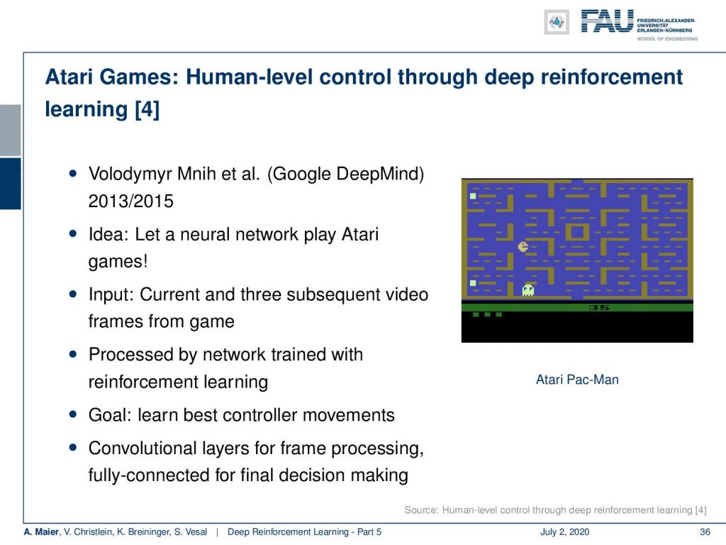
One of the very well-known examples is human-level control through deep reinforcement learning. Here in [4], this was done by Google Deepmind. They showed a neural network is able to play Atari games. So, the idea here is to directly learn the action-value function using a deep network. The inputs are essentially the three subsequent video frames from the game and this is processed by a deep network. It produces the best next action. So, the idea is now to use this deep reinforcement framework to learn the best next controller movements. They do convolutional layers for the frame processing and then fully connected layers for the final decision-making.
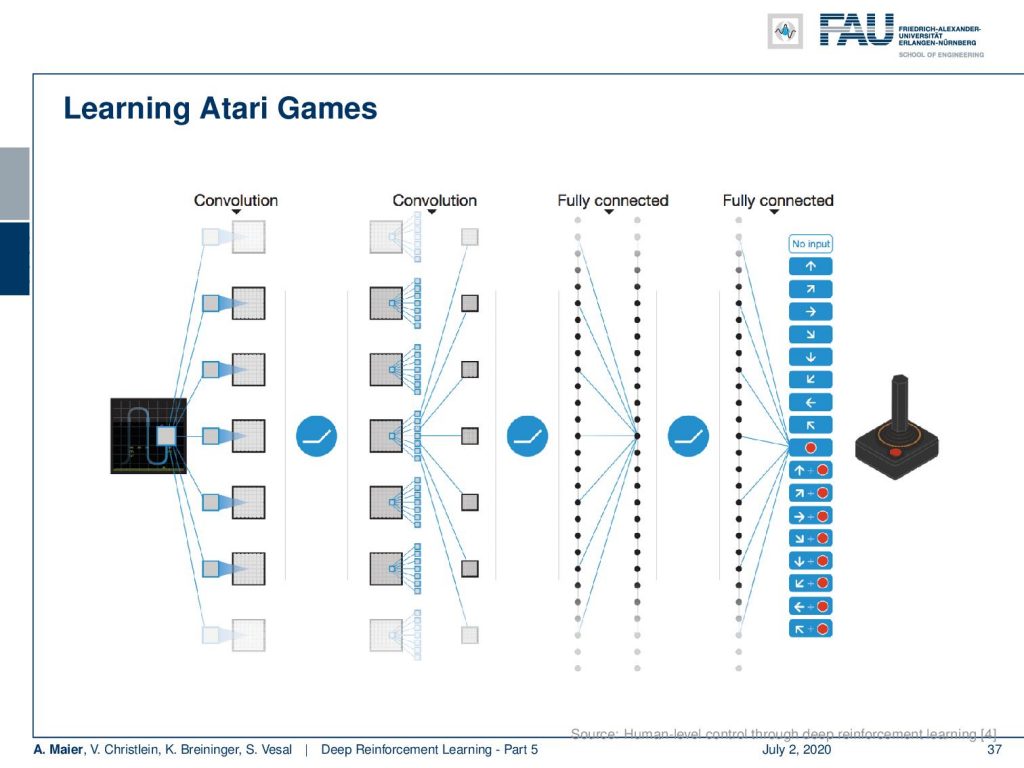
Here, you see the main idea of the architecture. So there are these convolutional layers and ReLUs. You have the input frames that are processed by these. Then, you go into fully connected layers and again fully connected layers. Finally, you produce directly the output and you can see that in Atari games this is a very limited set. So you can either do no action, then there are essentially eight directions, there’s a fire button, and there are eight directions plus the fire button. So that’s all of the different things that you can do. So, it’s a limited domain and you can then train your system with that.
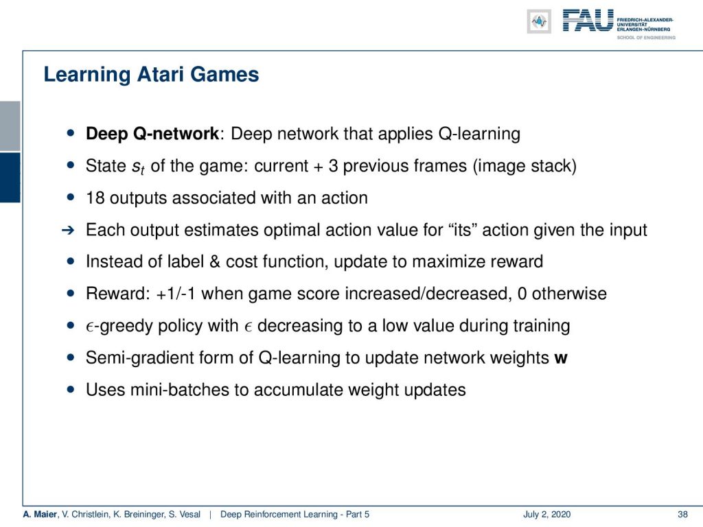
Well, it’s a deep network that directly applies Q-learning. The state of the game is essentially the current plus three previous frames as an image stack. So, you have a rather fuzzy way of incorporating memory and state. Then, you have 18 outputs that are associated with the different actions and each output estimates the action for the given input. You don’t have a label and a cost function, but you update with respect to maximize the future reward. There’s a reward of +1 when the game score is increased and a reward of -1 when the game score is decreased. Otherwise, it’s zero. They use an ε-greedy policy with ε decreasing to a low value during the training. They use a semi-gradient form of the Q-learning to update the network weights w and again they use mini-batches to accumulate the weight updates.
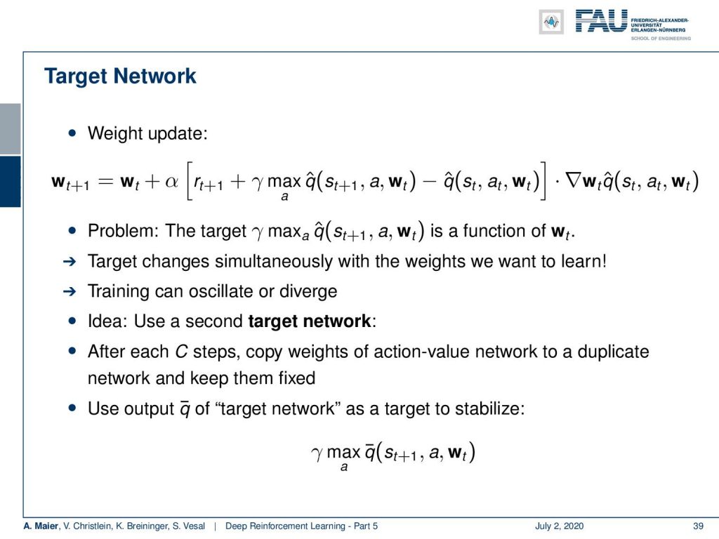
So, they have this target network and it’s updated using the following rule (see slide). You can see that this is very close to what we have seen in the previous video. Again, you have the weights and you update them with respect to the rewards. Now, the problem is, of course, that this γ and selection of the maximum q function is a function of the weights again. So, you now have a dependency on the maximization on the weights that you’re trying to update. So, your target changes simultaneously with the weights that we want to learn. This can actually lead to oscillations or divergence of your weights. So, this is not very good. To solve the problem, they introduce a second target network. After C steps, they generate this by copying the weights of the action-value network to a duplicate network and keep them fixed. So, you use the output q bar of the target network as a target to stabilize the previous maximization. You don’t use q hat, the function that you’re trying to learn, but you use the q bar which is the kind of fixed version that you use for a couple of iterations.
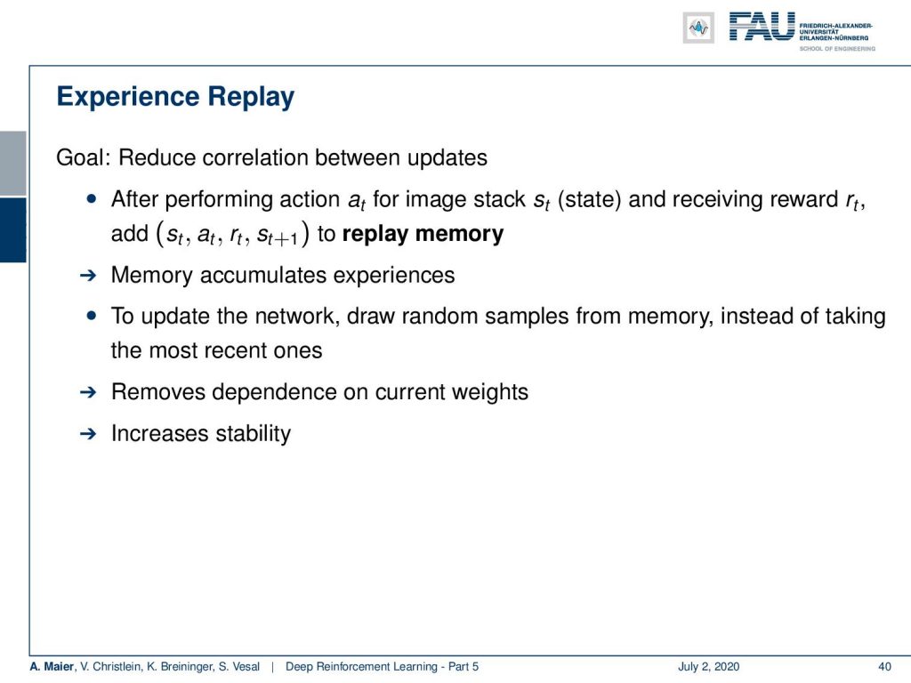
Another trick they have been using is experience replay. Here, the idea is to reduce the correlation between the updates. So after performing an action a subscript t for the image stack and receiving the reward, you add this to the replay memory. You accumulate experiences in this replay memory and then you update the network with samples drawn randomly from this memory instead of taking the most recent ones. This way, you kind of can stabilize and simultaneously not too much focus on one particular situation of the game. You try to keep in mind all of the different situations of the game and this removes the dependence on the current weights and increases the stability. I have a small example for you.
So, this is the Atari breakout game and you can see that the agent, in the beginning, is not performing very well. If you train it over several iterations, you can see that the game is played better. So the system learns how to follow with the paddle the ball and then it is able to reflect it. You can see that if you iterate and iterate, you could argue that at some point the reinforcement learning system also figures out the weaknesses of the game. In particular, one situation where you can score really a large number of points is if you manage to bring the ball behind the bricks and then have them jump around there. It will be reflected by the boundaries and not by the paddle and it will generate a large score. So, this is something that offers the claim that the system has learned to be a good strategy by trying to kick out only the bricks on the left-hand side. Then, it needs to get the ball into the region behind the other bricks.
Of course, we need to talk about AlphaGo in this video. We want to look into some of the details of how it’s actually implemented. You already heard about this one. So it’s from the paper mastering the game of go with deep neural networks.
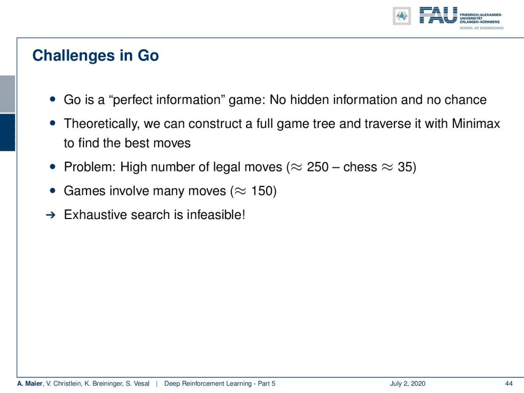
So, we already discussed that go is a much harder problem than chess because it really has a large number of possible moves. With also a large number of possible states that can potentially emerge, the idea is that black plays against white for the control over the board. It has simple rules but an extremely high number of possible moves and situations. To achieve the performance of human players was thought to be years away because of the high in numerical complexity of the problem. So, we could brute-force chess but with Go people thought it would be impossible until we have much much faster computers – orders of magnitude faster computers. They could show that they can really beat human Go experts with the system. So, Go is a perfect information game. There is no hidden information and no chance. So theoretically, we could construct a full game tree and traverse it with min-max to find the best moves. The problem is the high number of legal moves. So in chess, you have approximately 35. In Go, there are like 250 different moves that you can do during the game in each step.
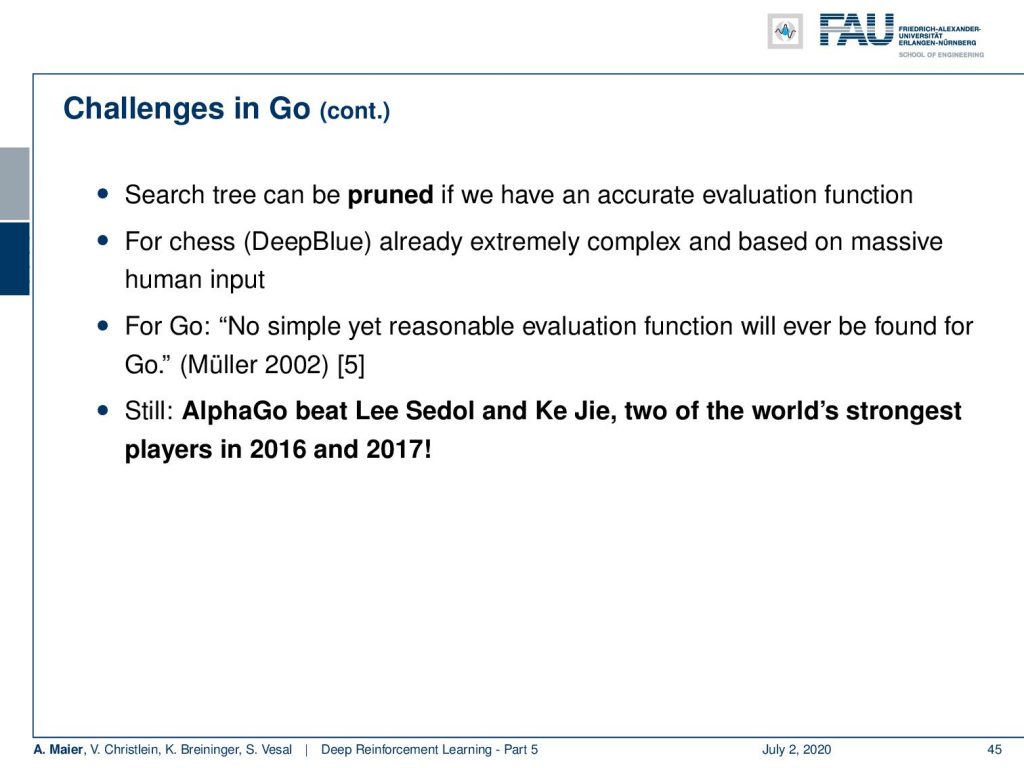
Also, the game may involve many moves. So approximately a hundred and fifty. This means that the exhaustive search is completely infeasible. Well, a search tree can, of course, be pruned if you have an accurate evaluation function. for chess, if you remember deep blue, this was already extremely complex and based on massive human input. Fo Go in 2002, “No simple yet reasonable evaluation will ever be found for Go.” was the state-of-the-art. Well in 2016 and 2017; AlphaGo beat Lee Sedol and Ke Kie, two of the world’s strongest players. So, there is a way of solving this game.
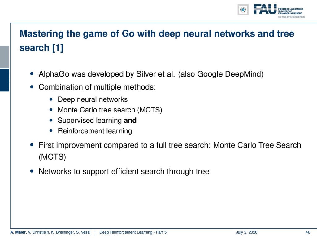
There were several very good ideas in this paper. It has been developed by Silver et al. It also Deepmind and it’s a combination of multiple methods. They use, of course, deep neural networks. Then, they use Monte Carlo Tree Search and they combine supervised learning and reinforcement learning. The first improvement compared to a full tree search was the Monte Carlo tree search. They use the networks to support efficient search through the tree.
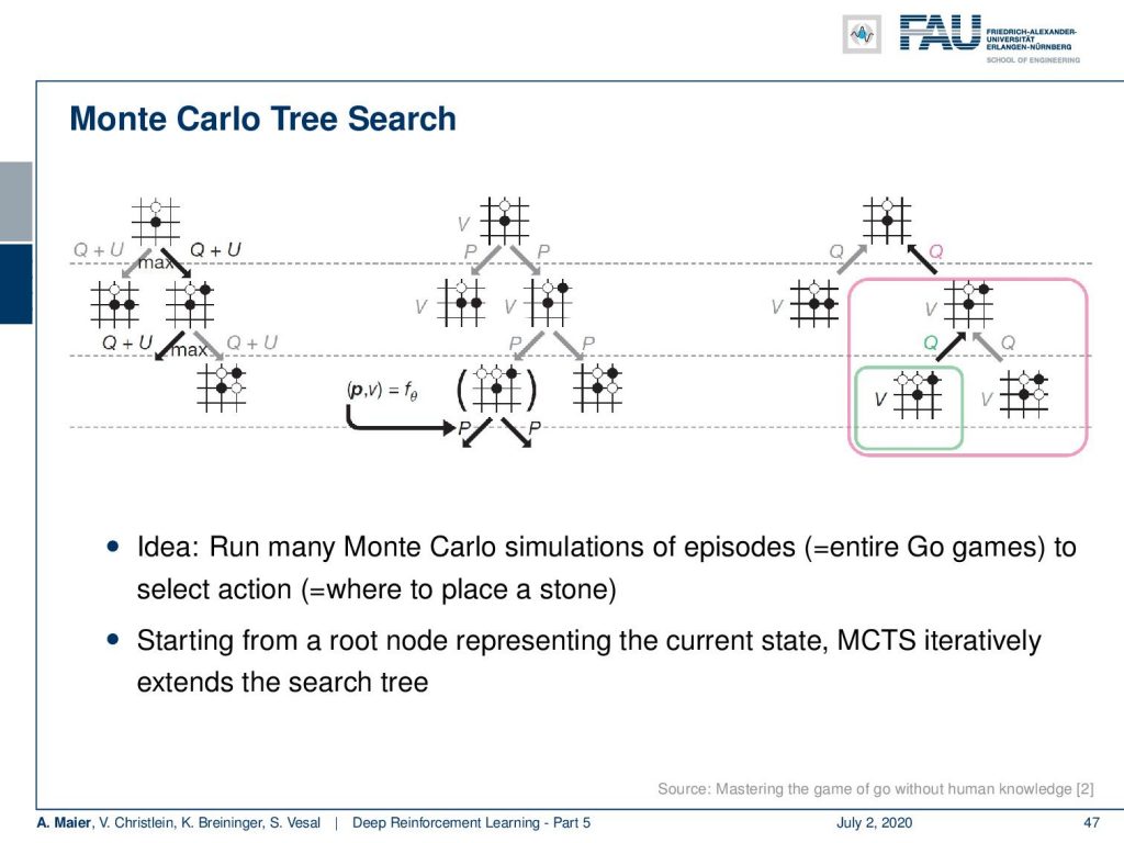
So, what’s Monte Carlo Tree Search? Well, you expand your tree by looking into different possible future moves and you look into the moves that produce very valuable states. You expand on the valuable state over a couple of moves into the future. Then, you also look at the value of these states. So you only look into a couple of valuable states and then expand over and over again for a couple of moves. Finally, you can find a situation where you probably have a much larger state value. So, you try to look a bit into the future and follow moves that are likely produced a higher state value.
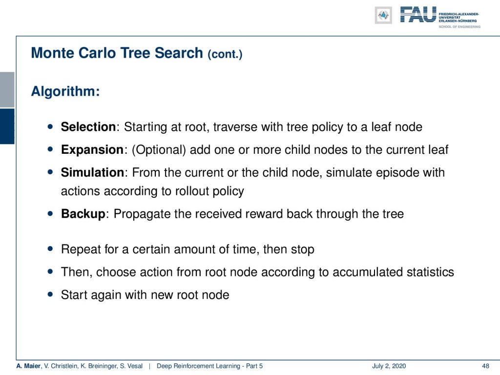
So, you start from the root node which is the current state. Then, you iteratively do that until you extend the search tree to find the best future state. Here’s the algorithm: you start at the root, you traverse with the tree policy to a leaf node. Then, you expand and you add one or more child nodes to the current leaf, probably the ones that have valuable states. Next, you simulate from the current or the child node, the episodes with actions according to your rollout policy. So, you also need a policy in order to expand here. Then, you can back up and propagate the received rewards backward through the tree. This allows you to find future states that have a large state value. So, you repeat that for a certain amount of time. Lastly, you stop and you choose the action from the root note according to the accumulated statistics. In the next move, you have to start again with a new root note according to the action that actually your opponent has taken.
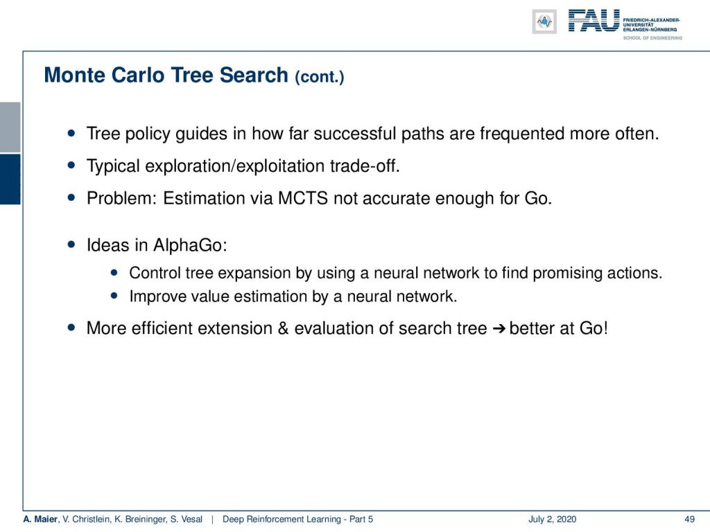
So the tree policy guides in how far successful paths are used and how frequently they will be looked at. This is a typical exploration/exploitation trade-off. Well, the main problem here is, of course, that the normal Monte Carlo Tree Search is not accurate enough for Go. The idea in AlphaGo was to control the tree expansion with a neural network to find promising actions and then improve the value estimation by a neural network. So, this is more efficient in terms of extension and evaluation than the search of a tree and this means that you better let go.
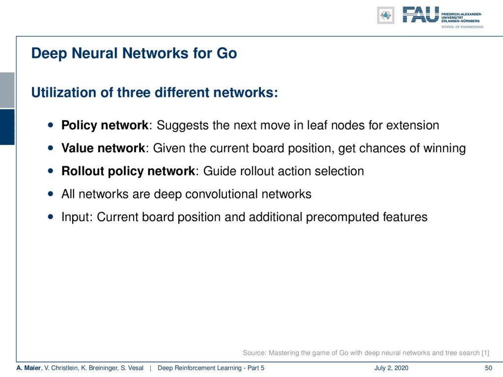
How do they use these deep neural networks? They have three different networks. They have a policy network that suggests the next move in a leaf node for the extension. Then they have a value network that looks at the current board situation and computes essentially the chances of winning. Lastly, they have a rollout policy network that guides the rollout action selection. All of those networks are deep convolutional networks and the input is the current board position and additional pre-computed features.
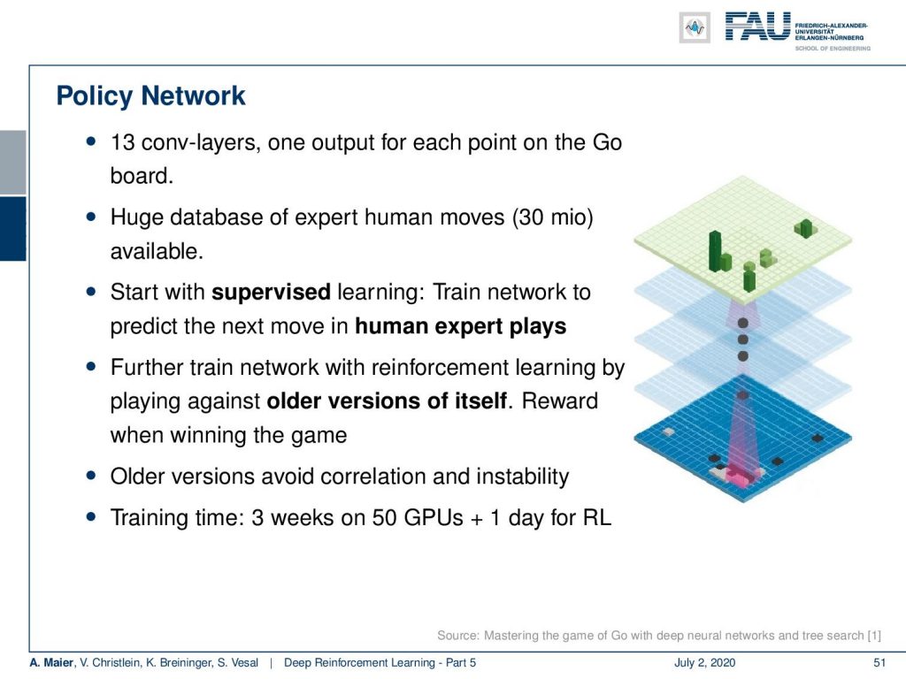
So, here’s the policy network. It had 13 convolutional layers one output for each point on the Go board. Then, a huge database of human expert moves, 30 million, that were available. They start with supervised learning and trained the network to predict the next move in the human expert play. Then, they train this network also with reinforcement learning by playing against older versions of the self and they have a reward for winning the game. All the versions, of course, avoid correlation instability. If you look at the training time, there were three weeks on 50 GPUs for the supervised part and one day for the reinforcement learning. So, actually quite a bit of supervised learning involved here – not so much reinforcement learning.
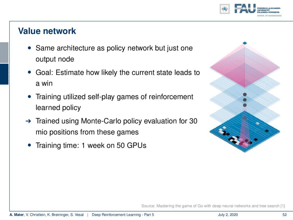
There’s the value network. This has the same architecture as the policy network, but just one output node. The goal is here to predict the probability of winning the game. They train again on self-play games of reinforcement learning and use Monte Carlo policy evaluation for 30 million positions from these games. Training time was one week on 50 GPUs.
Then, they have the rollout policy network that could then be used to select the moves during rollout. Of course, here, the problem is that the inference time is comparatively high and the solution was to train a simpler linear network on a subset of the data that provides actions very quickly. So, this led to a speed-up of approximately a thousand compared to the policy network. So if you work with this rollout policy network, then you have a slimmer network, but it’s much faster. So, you can do more simulations and collect more experience. So, this is why they use this rollout policy network.
Now, there was quite a bit of supervised learning involved here. So, let’s have a look at AlphaGo zero. Now, AlphaGo zero doesn’t need human play anymore. So, the idea here is that you then play solely with reinforcement learning and self-play. It has simpler Monte Carlo Tree Search and no rollout policy network in the Monte Carlo Tree Search. Also, in the self-play games, they also introduced multi-task learning. So, the policy and value network shared the initial layers. This then led to [3] and the extensions are also able to play chess and shogi. So, it’s not just code that can solve Go. With this, you can also play chess and shogi at an expert level. Okay. So, this sums up what we’ve been doing in reinforcement learning. Of course, we could look at many other things here. However, there is just not enough time.
Next time in deep learning, we want to talk about algorithms that even don’t have rewards. So, complete unsupervised training and we also want to learn how to benefit from adversaries. We will see that there’s a very cool concept out there that is called generative adversarial networks which is able to generate all kinds of different images. Also, a very cool concept that we’ll talk about in one of the next videos, Then we look into extensions into performing image processing tasks. So, we go more and more towards the applications.
Well, some comprehensive questions: What is a policy? What are value functions? Explain the exploitation versus exploration dilemma, and so on. If you’re interested in reinforcement learning, I can definitely recommend having a look at the book reinforcement learning by Richard Sutton. It’s really a great book and you will learn in high detail about all the things that we could only scratch on in these videos. So, you see that you can go much deeper into all of the details of reinforcement learning and also deep reinforcement learning. There’s actually much more to say about this at this point, but we can only remain at this level for the time being. Well, I also brought you the link and I put also the link into the video description. So please enjoy this book it’s very good and, of course, we have plenty of further references.
So, thank you very much for listening and I hope you that you can now understand at least in a bit of what is happening in reinforcement learning and deep reinforcement learning and what the main ideas are in order to perform learning of games. So, thank you very much for watching this video and hope to see you in the next one. Bye-bye!
If you liked this post, you can find more essays here, more educational material on Machine Learning here, or have a look at our Deep LearningLecture. I would also appreciate a follow on YouTube, Twitter, Facebook, or LinkedIn in case you want to be informed about more essays, videos, and research in the future. This article is released under the Creative Commons 4.0 Attribution License and can be reprinted and modified if referenced. If you are interested in generating transcripts from video lectures try AutoBlog.
Links
Link to Sutton’s Reinforcement Learning in its 2018 draft, including Deep Q learning and Alpha Go details
References
[1] David Silver, Aja Huang, Chris J Maddison, et al. “Mastering the game of Go with deep neural networks and tree search”. In: Nature 529.7587 (2016), pp. 484–489.
[2] David Silver, Julian Schrittwieser, Karen Simonyan, et al. “Mastering the game of go without human knowledge”. In: Nature 550.7676 (2017), p. 354.
[3] David Silver, Thomas Hubert, Julian Schrittwieser, et al. “Mastering Chess and Shogi by Self-Play with a General Reinforcement Learning Algorithm”. In: arXiv preprint arXiv:1712.01815 (2017).
[4] Volodymyr Mnih, Koray Kavukcuoglu, David Silver, et al. “Human-level control through deep reinforcement learning”. In: Nature 518.7540 (2015), pp. 529–533.
[5] Martin Müller. “Computer Go”. In: Artificial Intelligence 134.1 (2002), pp. 145–179.
[6] Richard S. Sutton and Andrew G. Barto. Introduction to Reinforcement Learning. 1st. Cambridge, MA, USA: MIT Press, 1998.