Lecture Notes in Deep Learning: Segmentation and Object Detection – Part 4

Single Shot Detectors

These are the lecture notes for FAU’s YouTube Lecture “Deep Learning“. This is a full transcript of the lecture video & matching slides. We hope, you enjoy this as much as the videos. Of course, this transcript was created with deep learning techniques largely automatically and only minor manual modifications were performed. Try it yourself! If you spot mistakes, please let us know!

Welcome back to deep learning! So today, we want to discuss the single-shot detectors and how we can actually approach real-time object detection.

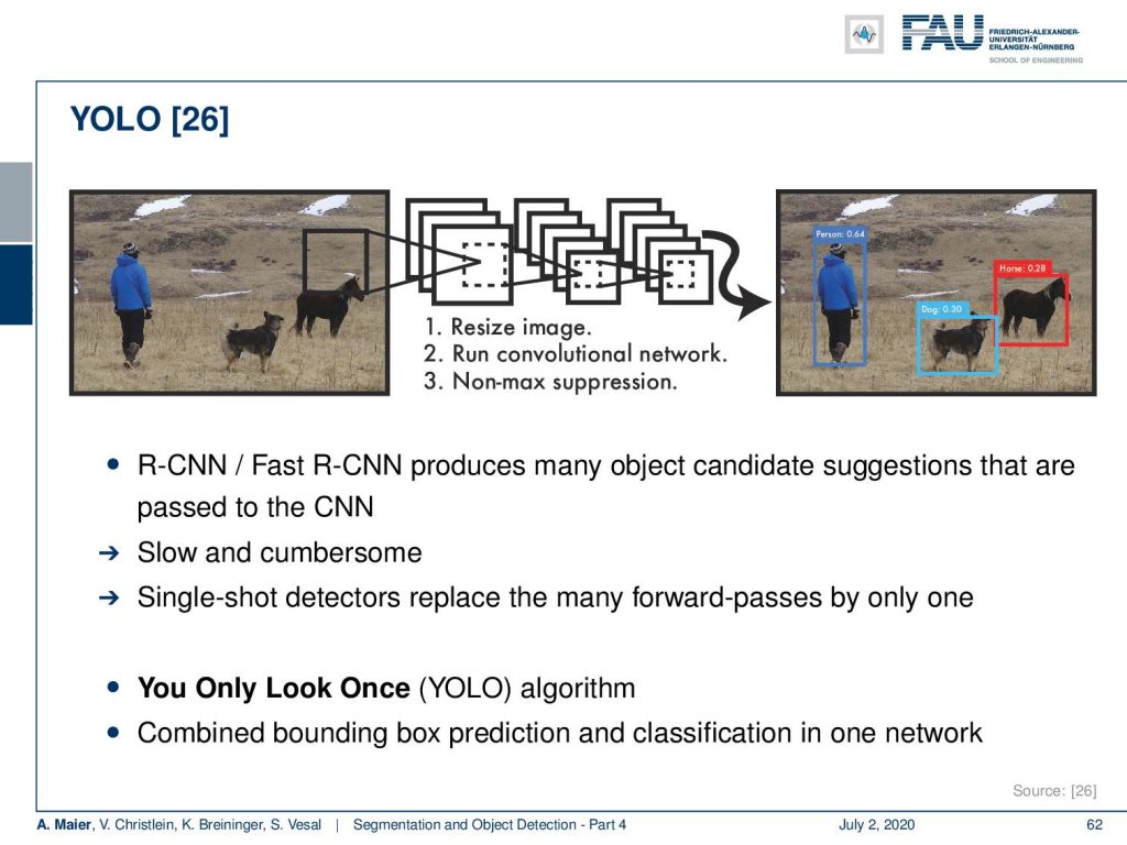
Okay, the fourth part of segmentation and object detection – the single-shot detectors. So, can’t we just use the region proposal network as a detector in you look only once fashion? This is the idea of YOLO that is a single-shot detector. You only look once – you combine the bounding box prediction and the classification into a single network.

This is done by subdividing the image essentially into S times S cells and for every cell, you do in parallel the class probability map computation and you produce bounding boxes and confidence. This then gives you for each cell B bounding boxes with a confidence score and the class confidence and that is produced from a CNN. So the CNN predicts S times S times (5 B + C) values, where C is the number of classes. In the end, to produce the final object detection, you compute the overlap of the bounding box with the respective class probability map. This then allows you to compute the average within this bounding box to produce the final class of that respective object. This way you are able to solve complex scenes like this one and this is really real-time.

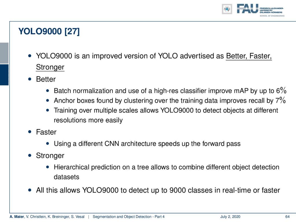
So there’s YOLO9000 which is an improved version of YOLO which is advertised as better, faster, and stronger. So it’s better because the batch normalization is used. They also do high-res classification to improve the mean average precision by up to 6%. The anchor boxes that are found by the clustering over the training data improves the recall by 7%. Training over multiple scales allows YOLO9000 to detect objects at different resolutions more easily. It’s faster because it’s using a difference CNN architecture which speeds up the forward pass. Finally, it’s stronger because it has this hierarchical detection on a tree that allows combining different object detection datasets. All in this allows YOLO9000 to detect up to 9,000 classes in real-time or faster.

There is also the single-shot multi-box detector in [24]. It’s a popular alternative to YOLO. It is also a single-shot detector like Yolo with only one forward pass through the CNN.

It’s called multi-box because this is the name of the bounding box regression technique in [15] and it’s obviously an object detector. It differs from YOLO in several aspects but shares the same core idea.

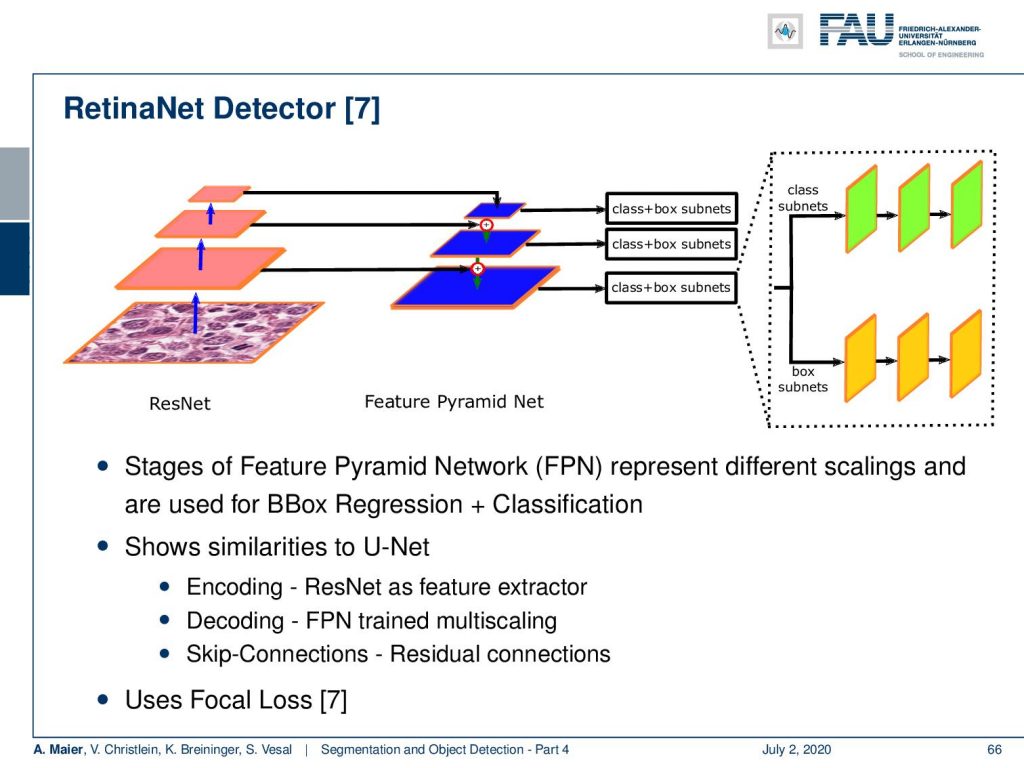
Now, you still have a problem with multiple resolutions. In particular, if you think about tasks like histological images that have a very, very high resolution. Then, you can also work with detectors like RetinaNet. It is essentially using a ResNet CNN encoder/decoder. It’s very similar to what we’ve already seen in image segmentation. It’s using a feature pyramid net that allows you to couple the different feature maps that are produced with the original input images that are generated from the decoder. So you could say it’s very similar to a U-net. In contrast to U-net, it does a class and box prediction using a subnet on each of the scales of the feature pyramid net. So, you could say it’s a single-shot detector that uses U-net simultaneously for the class and box prediction. Also, it uses the focal loss that we will talk about in a couple of slides.

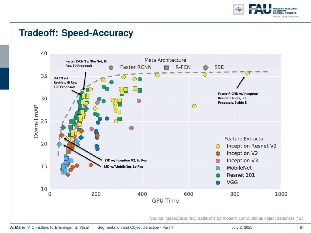
Let’s look a bit at the tradeoff in speed and accuracy. You can see that generally, networks that are very accurate are not so fast. So, here you see on the x-axis the GPU time and on the y-axis the overall mean average precision. You can see that you can combine the architectures like single-shot detectors, RCNN, or ideas like faster RCNN in combination with different feature extractors like Inception-ResNet, Inception, and so on. This allows us to produce many different combinations. You can see that if you spend more time on the computation, then you typically can also increase the accuracy and this is reflected in this graph.

The class imbalance is key to tackle the speed-accuracy tradeoff. All of those single-shot detectors evaluate many hypothesis locations. Most of them are really easy negatives. So, this imbalance is not addressed by the current training. In classical methods, we typically dealt with this with hard-negative mining. Now, the question is “Can we change the loss function to pay less attention to easy examples?”.

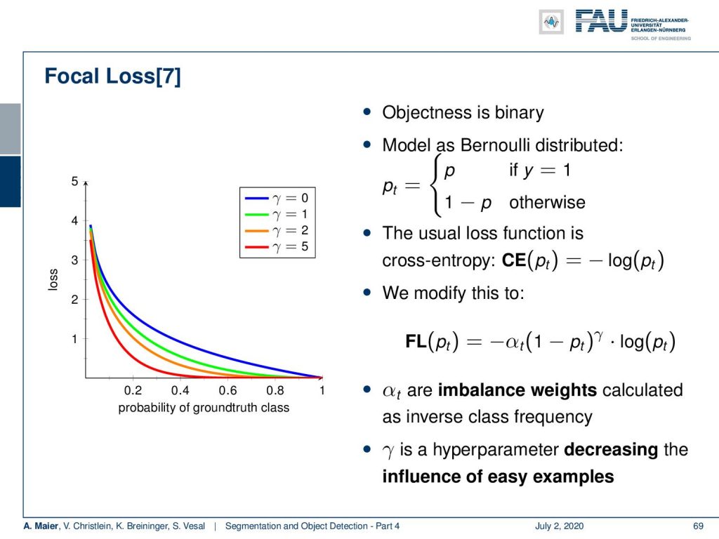
This idea exactly brings us to the focal loss. Here, we can essentially define the objectness whether it’s an object or not as binary. Then, you can model this as a Bernoulli distribution. The usual loss would be simply the cross-entropy where you have the minus logarithm of the correct class. You can now see that we can adjust this to the so-called focal loss. Here, we introduce an additional parameter α. α is the imbalance weight calculated as the inverse class frequency. Additionally, we introduced some γ that is a hyper-parameter. This allows decreasing the influence of easy examples. So, you can see the influence of γ here on the plot on the left-hand side. The more you increase γ is the more peaked will your respective weight be such that you can then really concentrate on classes that are not very frequent.

So, let’s summarize object detection. The main task is detecting bounding boxes and associated classification. The sliding window approach was extremely inefficient. The region proposal networks reduce the number of candidates but if you really want to go towards real-time then you have to use single-shot detectors like YOLO to avoid additional steps. Object detector concepts can, of course, be combined with arbitrary feature extraction and classification networks as we’ve seen earlier. Also, keep in mind the speed-accuracy tradeoff. So, if you want to be very quick then you, of course, reduce the number of bounding boxes that are predicting because then you are much faster but then you may miss true positives.

So, we now discussed segmentation. We now discussed object detection and how to do object detection very quickly. So next time, we will look into the fusion of both which is going to be instance segmentation. So, thank you very much for watching this video and I’m looking forward to seeing you in the next one.

If you liked this post, you can find more essays here, more educational material on Machine Learning here, or have a look at our Deep LearningLecture. I would also appreciate a follow on YouTube, Twitter, Facebook, or LinkedIn in case you want to be informed about more essays, videos, and research in the future. This article is released under the Creative Commons 4.0 Attribution License and can be reprinted and modified if referenced. If you are interested in generating transcripts from video lectures try AutoBlog.

References

[1] Vijay Badrinarayanan, Alex Kendall, and Roberto Cipolla. “Segnet: A deep convolutional encoder-decoder architecture for image segmentation”. In: arXiv preprint arXiv:1511.00561 (2015). arXiv: 1311.2524.
[2] Xiao Bian, Ser Nam Lim, and Ning Zhou. “Multiscale fully convolutional network with application to industrial inspection”. In: Applications of Computer Vision (WACV), 2016 IEEE Winter Conference on. IEEE. 2016, pp. 1–8.
[3] Liang-Chieh Chen, George Papandreou, Iasonas Kokkinos, et al. “Semantic Image Segmentation with Deep Convolutional Nets and Fully Connected CRFs”. In: CoRR abs/1412.7062 (2014). arXiv: 1412.7062.
[4] Liang-Chieh Chen, George Papandreou, Iasonas Kokkinos, et al. “Deeplab: Semantic image segmentation with deep convolutional nets, atrous convolution, and fully connected crfs”. In: arXiv preprint arXiv:1606.00915 (2016).
[5] S. Ren, K. He, R. Girshick, et al. “Faster R-CNN: Towards Real-Time Object Detection with Region Proposal Networks”. In: vol. 39. 6. June 2017, pp. 1137–1149.
[6] R. Girshick. “Fast R-CNN”. In: 2015 IEEE International Conference on Computer Vision (ICCV). Dec. 2015, pp. 1440–1448.
[7] Tsung-Yi Lin, Priya Goyal, Ross Girshick, et al. “Focal loss for dense object detection”. In: arXiv preprint arXiv:1708.02002 (2017).
[8] Alberto Garcia-Garcia, Sergio Orts-Escolano, Sergiu Oprea, et al. “A Review on Deep Learning Techniques Applied to Semantic Segmentation”. In: arXiv preprint arXiv:1704.06857 (2017).
[9] Bharath Hariharan, Pablo Arbeláez, Ross Girshick, et al. “Simultaneous detection and segmentation”. In: European Conference on Computer Vision. Springer. 2014, pp. 297–312.
[10] Kaiming He, Georgia Gkioxari, Piotr Dollár, et al. “Mask R-CNN”. In: CoRR abs/1703.06870 (2017). arXiv: 1703.06870.
[11] N. Dalal and B. Triggs. “Histograms of oriented gradients for human detection”. In: 2005 IEEE Computer Society Conference on Computer Vision and Pattern Recognition Vol. 1. June 2005, 886–893 vol. 1.
[12] Jonathan Huang, Vivek Rathod, Chen Sun, et al. “Speed/accuracy trade-offs for modern convolutional object detectors”. In: CoRR abs/1611.10012 (2016). arXiv: 1611.10012.
[13] Jonathan Long, Evan Shelhamer, and Trevor Darrell. “Fully convolutional networks for semantic segmentation”. In: Proceedings of the IEEE Conference on Computer Vision and Pattern Recognition. 2015, pp. 3431–3440.
[14] Pauline Luc, Camille Couprie, Soumith Chintala, et al. “Semantic segmentation using adversarial networks”. In: arXiv preprint arXiv:1611.08408 (2016).
[15] Christian Szegedy, Scott E. Reed, Dumitru Erhan, et al. “Scalable, High-Quality Object Detection”. In: CoRR abs/1412.1441 (2014). arXiv: 1412.1441.
[16] Hyeonwoo Noh, Seunghoon Hong, and Bohyung Han. “Learning deconvolution network for semantic segmentation”. In: Proceedings of the IEEE International Conference on Computer Vision. 2015, pp. 1520–1528.
[17] Adam Paszke, Abhishek Chaurasia, Sangpil Kim, et al. “Enet: A deep neural network architecture for real-time semantic segmentation”. In: arXiv preprint arXiv:1606.02147 (2016).
[18] Pedro O Pinheiro, Ronan Collobert, and Piotr Dollár. “Learning to segment object candidates”. In: Advances in Neural Information Processing Systems. 2015, pp. 1990–1998.
[19] Pedro O Pinheiro, Tsung-Yi Lin, Ronan Collobert, et al. “Learning to refine object segments”. In: European Conference on Computer Vision. Springer. 2016, pp. 75–91.
[20] Ross B. Girshick, Jeff Donahue, Trevor Darrell, et al. “Rich feature hierarchies for accurate object detection and semantic segmentation”. In: CoRR abs/1311.2524 (2013). arXiv: 1311.2524.
[21] Olaf Ronneberger, Philipp Fischer, and Thomas Brox. “U-net: Convolutional networks for biomedical image segmentation”. In: MICCAI. Springer. 2015, pp. 234–241.
[22] Kaiming He, Xiangyu Zhang, Shaoqing Ren, et al. “Spatial Pyramid Pooling in Deep Convolutional Networks for Visual Recognition”. In: Computer Vision – ECCV 2014. Cham: Springer International Publishing, 2014, pp. 346–361.
[23] J. R. R. Uijlings, K. E. A. van de Sande, T. Gevers, et al. “Selective Search for Object Recognition”. In: International Journal of Computer Vision 104.2 (Sept. 2013), pp. 154–171.
[24] Wei Liu, Dragomir Anguelov, Dumitru Erhan, et al. “SSD: Single Shot MultiBox Detector”. In: Computer Vision – ECCV 2016. Cham: Springer International Publishing, 2016, pp. 21–37.
[25] P. Viola and M. Jones. “Rapid object detection using a boosted cascade of simple features”. In: Proceedings of the 2001 IEEE Computer Society Conference on Computer Vision Vol. 1. 2001, pp. 511–518.
[26] J. Redmon, S. Divvala, R. Girshick, et al. “You Only Look Once: Unified, Real-Time Object Detection”. In: 2016 IEEE Conference on Computer Vision and Pattern Recognition (CVPR). June 2016, pp. 779–788.
[27] Joseph Redmon and Ali Farhadi. “YOLO9000: Better, Faster, Stronger”. In: CoRR abs/1612.08242 (2016). arXiv: 1612.08242.
[28] Fisher Yu and Vladlen Koltun. “Multi-scale context aggregation by dilated convolutions”. In: arXiv preprint arXiv:1511.07122 (2015).
[29] Shuai Zheng, Sadeep Jayasumana, Bernardino Romera-Paredes, et al. “Conditional Random Fields as Recurrent Neural Networks”. In: CoRR abs/1502.03240 (2015). arXiv: 1502.03240.
[30] Alejandro Newell, Kaiyu Yang, and Jia Deng. “Stacked hourglass networks for human pose estimation”. In: European conference on computer vision. Springer. 2016, pp. 483–499.

Category: Lecture Notes in Deep Learning