Lecture Notes in Deep Learning: Segmentation and Object Detection – Part 3

A Family of Regional CNNs

These are the lecture notes for FAU’s YouTube Lecture “Deep Learning“. This is a full transcript of the lecture video & matching slides. We hope, you enjoy this as much as the videos. Of course, this transcript was created with deep learning techniques largely automatically and only minor manual modifications were performed. Try it yourself! If you spot mistakes, please let us know!

Welcome back to deep learning! So today, we want to talk a bit more about the ideas of object detection. We will start with a small motivation on object detection and some key ideas on how this can actually be performed.

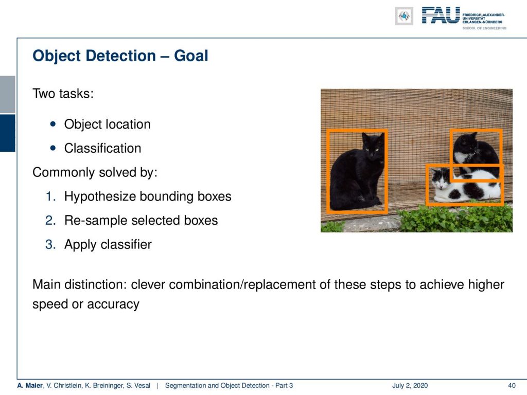
So, let’s have a look at our slides. You see this is already part three of our short lecture video series on segmentation and object detection. Now, the topic is object detection. Well, let’s motivate this a little bit. The idea – you remember – is that we want to localize objects and we classify them. So, we want to figure out where the cats are in the image and we want to figure out whether they are actually cats. This is then commonly solved by generating hypotheses about bounding boxes, then you resample those boxes, and apply a classifier. So the main distinction of the methods is how you combine and replace those steps in order to achieve higher speed or accuracy.

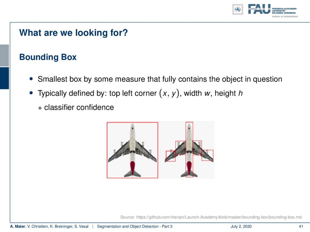
We can also look into this plane example. Of course, we are looking for bounding boxes and the bounding boxes are typically defined as the smallest box that fully contains the object in question. This is then typically defined as a top-left corner with width w and height h and some classifier confidence for the bounding box. You can see that we can also use this for detecting the entire plane or we could also use it for parts of the plane.

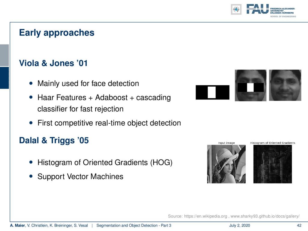
This is actually something where we already have a long history of different success stories. One very early successor is the Viola and Jones algorithm that was one of the earliest really well-working face detectors. Here you can see the example. This was using Haar-features and those Haar-features were then used in a kind of boosting cascade in order to detect faces very quickly. So, it was using large numbers of features that can be computed very efficiently. Then in the boosting cascade, they would select only the features that are most likely to detect a face at a given position. This was then improved with the so-called histogram of oriented gradients and in classical methods. You had always a good feature extraction plus some effective classification. At the time, support vector machines were very common.

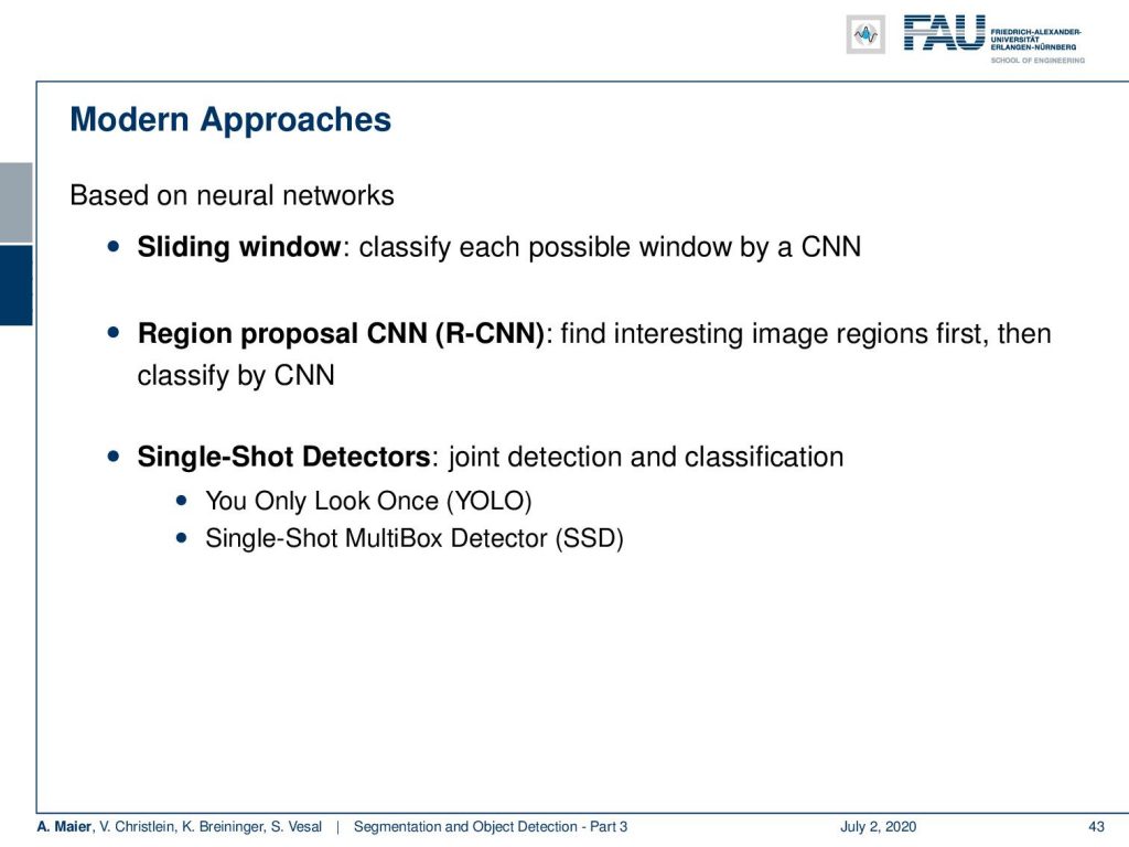
Of course, there are also neural network-based approaches. You can do this actually quite easily with a pre-trained CNN. So, you could simply use the sliding window approach and then detect each possible window by a CNN. There are region proposal CNNs like RCNN that find interesting image regions first and then classifies them with our CNN. There are single-shot detectors that we talk about in the next video that do a joint detection and classification. I think one of the most famous examples is YOLO – you only look once – we already had that example also in the introduction. It’s a very nice method that does all of these detection approaches in real-time.

Well, in the sliding window approaches, you could simply take your pre-trained CNN and just move it all across the image. When you find an area of high confidence, you could say: “Okay. There is a face and I want to detect this face!” Now, the big disadvantage here is that you have not just to detect the face but the face could also be at different resolutions. So, you want to repeat this process on multiple resolutions. Then, you already see that detecting patch-wise will result in a large number of patches. You have to do a large number of classifications. So, this is probably not the way that we want to go. One advantage, of course, would be that we don’t need to train anew. We can simply use our trained classification network in this case. But it’s computationally very inefficient and we want to look for some ideas on how to do that more efficiently.

One idea is, of course, that you use it with fully convolutional neural networks and understand the following approach. So, we can think about the idea of how we could apply a fully connected layer to an arbitrary shape tensor. One idea would be that you flatten the activations then you run your fully connected layer and you can get one classification result. Instead, you can reshape your weights and then use convolution. This will produce exactly the same result. We already discussed this when we were talking about one-by-one convolutions. Now, the nice property here is that if we follow this idea, we can then also work with arbitrarily shaped spacial input sizes. By using the convolution, we will then also produce larger output sizes. So, we kind of get away with the moving window approach but we still have the problem that we would have to look at the different scales in order to find all of the interesting objects.

This is why people have been looking at region-based detectors. So, we know that CNNs are powerful classifiers and the fully convolutional neural networks help to improve efficiency. But they are still somewhat brute-force. So, what can we do about this? We can improve efficiency by only considering interesting regions like our eyes do. So, this then leads to RCNN, the regional CNN. So here, you have this multi-step approach where you generate region proposals and a selective search. Then, you classify the content of the region proposals within a refined bounding box.

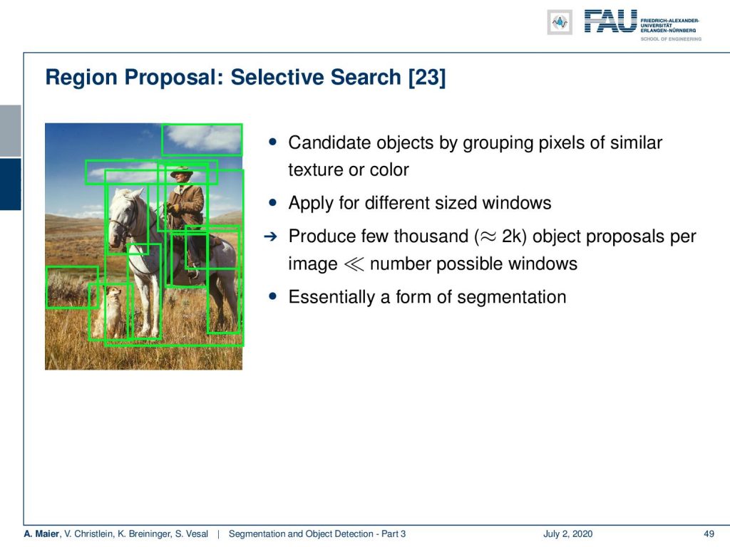
So let’s look at this in slightly more detail. Here, our region proposals, you generate those candidate objects by a grouping of pixels with similar texture and color. Then you produce a few thousand object proposals like two thousand per image. You note that this is much, much smaller than the number of possible windows. You essentially base this on a form of coarse segmentation.

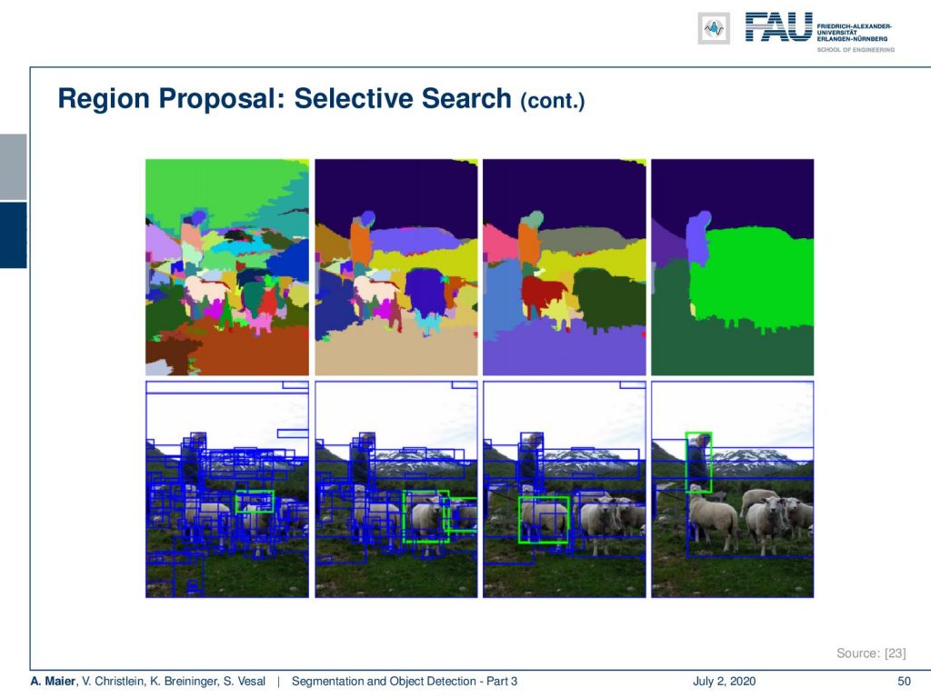
In the original RCNN paper, they were actually using a method called superpixels. Superpixels allow you to generate smaller and larger regions. So, you can see how we increase the region size from left to right. Then, we can use those regions in order to find interesting areas with another detector. These interesting areas can then be fed into the next stage of the classifier.

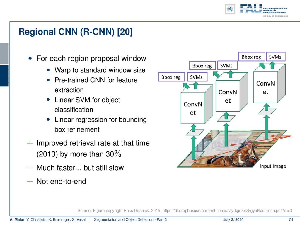
So, in the second stage – once we have those regions – we essentially have a convolutional neural network. This then produces, on the one hand, a box regression that refines the bounding box. On the other hand, this is then also fed as a kind of representation learning to a support vector machine that does the final decision. So this is better than what we’ve seen before at that time in 2013, but it’s still slow and it’s not end-to-end. So, if we want to accelerate this, then we see that we still have problems with RCNN.

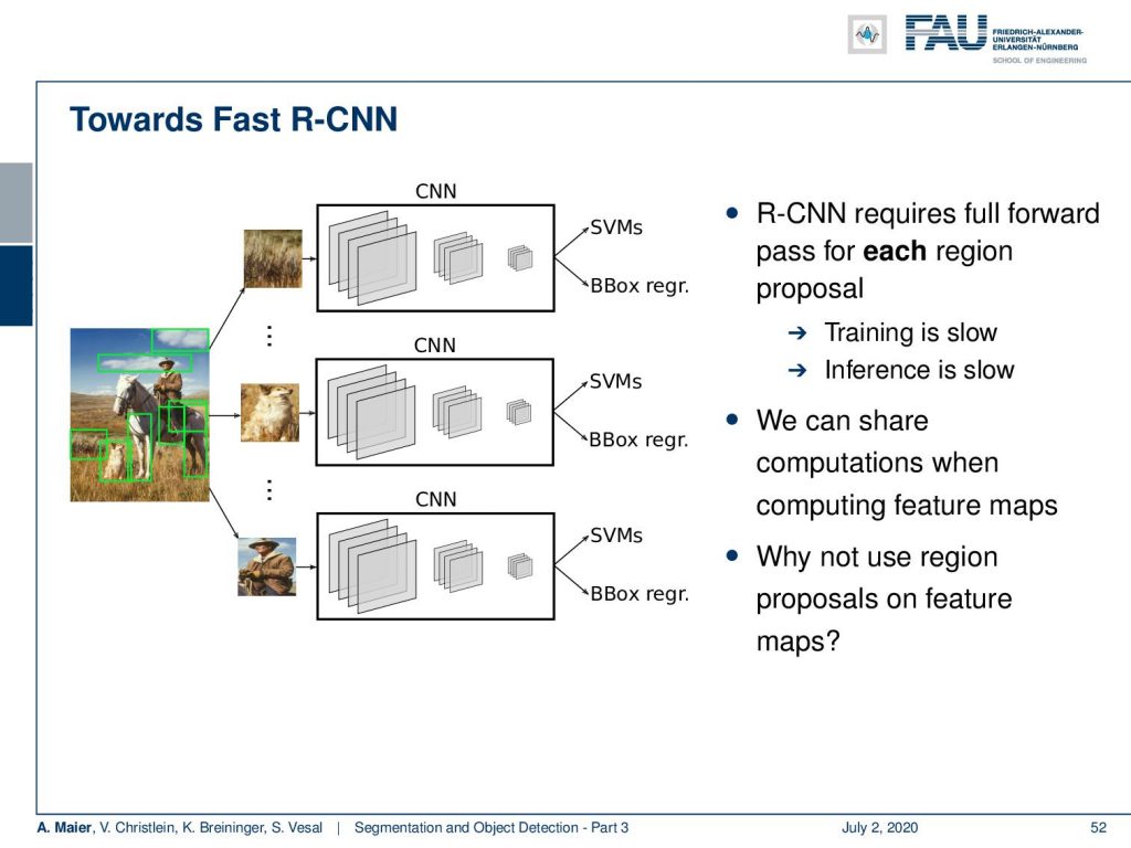
Because we had this full forward pass for each region proposal, this means that this training is slow, and also the inference is slow. We can share the computations when computing the feature maps because we’re doing the same or similar computations all along. Then, the key idea in order to improve the inference speed is that we use the region proposals on the feature maps.

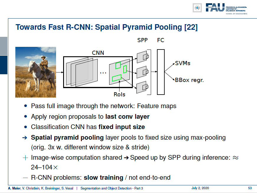
So, what you do is you pass the entire image through the network to generate feature maps. Then, you apply the region proposals to the last convolutional layer. Hence, you have to resize them in order to be applied to the layer. You can do that because you can predict the size of this particular layer by counting of the pooling steps to reformat the detected superpixels. The classification CNN has a fixed input size. So, you use the so-called spatial pyramid pooling to resample this to a fixed size using max-pooling. Originally this has been done with three different window sizes and strides. Then, you essentially have this image-wise computation shared and this gives a big speed up during the inference. You already can accelerate the inference by a factor of 24 to a104. Still, you have slow training which is not end-to-end.

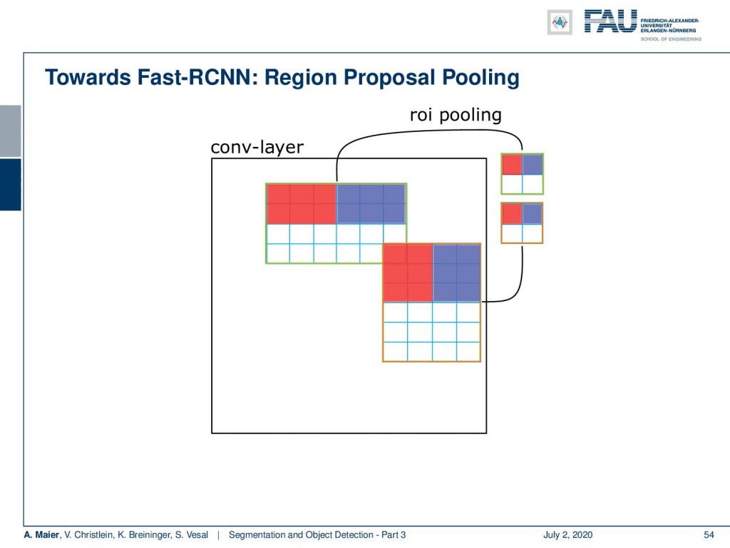
One reason is that we have this region proposal pooling where you pool according to these suggestions that you have from the region identification. You can do that simply with max-pooling. You lose a bit of information in this step if you just do it in a fixed sampling.

Also, this spatial pyramid pooling is used with one output map. They have some ideas to better sample the selection for the mini-batches. You can sample 128 ROIs uniform randomly and if you do that then typically the feature maps don’t overlap. Instead, you can also do hierarchical sampling that then samples from a few images but many ROIs, let’s say 64. Then, you generate a high overlap. You replace the support vector machine and the regression by a softmax layer for classification and a regression layer for the bounding box fine-tuning. This then leads to a multi-task loss and in total, the training is then nine times faster than RCNN. But we’re still not real-time. So we almost end-to-end apart from the ROI proposals.

So what you can do then in order to speed up further is the so-called faster RCNN. Here, the key idea is that you add a region proposal network, the input is now the generated feature maps and the output of our region proposals.

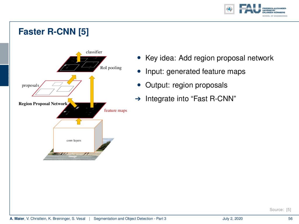
This is integrated into the fast RCNN. The idea here is that you define anchor boxes with different scale and aspect ratios, typically, three scales, and three aspect ratios. This leads to efficient multiscaling. So, neither the image sizes nor the filter sizes need to change. You get some 4,000 box parameters plus 2,000 scores because you have the softmax for object/non-object detection.

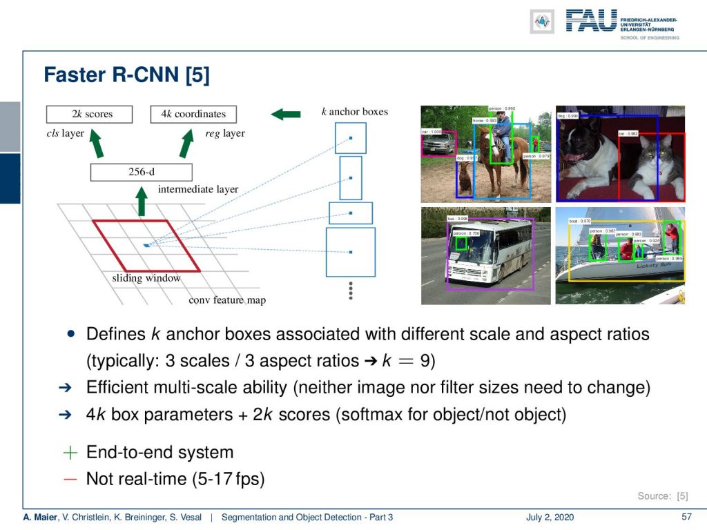
So, you then have a fully convolutional end-to-end system, but the system is still not real-time. So, let’s compare those approaches. Here you can see the overview of the different architectures based on RCNN.

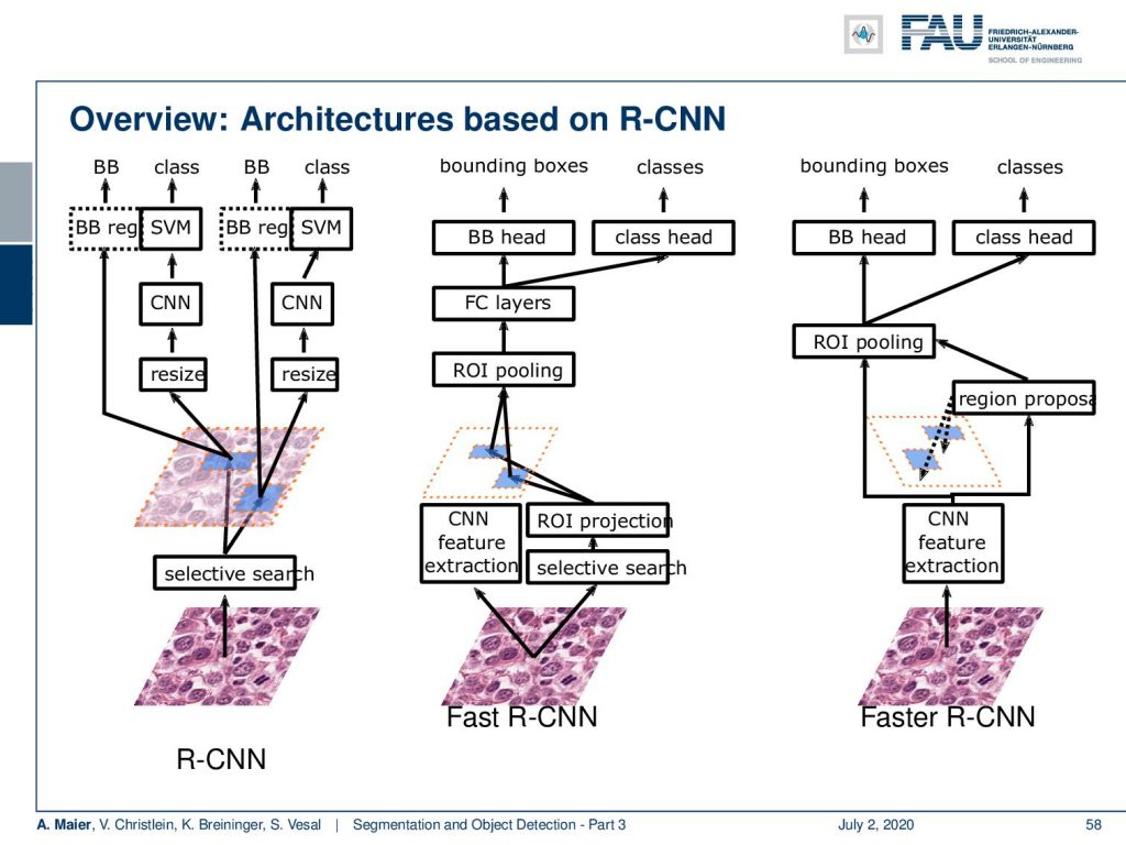
You see that RCNN itself was doing this selective search. Then, based on the selective search that produced the regions of interest, you then do a resizing. You use a CNN that is then processed by a support vector machine and you also do a bounding box regression to refine the bounding boxes. So, the fast RCNN is using one CNN for feature extraction in a fully convolutional approach. You have the entire feature maps that are produced in one step. You still have the selective search that is then generating ROIs and you can use them in the spatial pyramid pooling in order to feed your fully connected layers. Then, you have the bounding box detection head and the class head that is doing this kind of multi-task prediction. In faster RCNN, you go really into an end-to-end system. Here, you have the CNN feature extraction. From these extracted features, you do the region proposals. You do the ROI pooling subsequently and then you have the bounding box prediction head and the class head which is much faster in terms of training, end-to-end, and much faster in terms of inference.

Still, we are not able to do real-time classification which is why we want to talk next time about single-shot detectors that will be able to do this trick. I really hope you enjoyed this video and I’m looking forward to seeing you in the next one. Bye-bye!

If you liked this post, you can find more essays here, more educational material on Machine Learning here, or have a look at our Deep LearningLecture. I would also appreciate a follow on YouTube, Twitter, Facebook, or LinkedIn in case you want to be informed about more essays, videos, and research in the future. This article is released under the Creative Commons 4.0 Attribution License and can be reprinted and modified if referenced. If you are interested in generating transcripts from video lectures try AutoBlog.

References

[1] Vijay Badrinarayanan, Alex Kendall, and Roberto Cipolla. “Segnet: A deep convolutional encoder-decoder architecture for image segmentation”. In: arXiv preprint arXiv:1511.00561 (2015). arXiv: 1311.2524.
[2] Xiao Bian, Ser Nam Lim, and Ning Zhou. “Multiscale fully convolutional network with application to industrial inspection”. In: Applications of Computer Vision (WACV), 2016 IEEE Winter Conference on. IEEE. 2016, pp. 1–8.
[3] Liang-Chieh Chen, George Papandreou, Iasonas Kokkinos, et al. “Semantic Image Segmentation with Deep Convolutional Nets and Fully Connected CRFs”. In: CoRR abs/1412.7062 (2014). arXiv: 1412.7062.
[4] Liang-Chieh Chen, George Papandreou, Iasonas Kokkinos, et al. “Deeplab: Semantic image segmentation with deep convolutional nets, atrous convolution, and fully connected crfs”. In: arXiv preprint arXiv:1606.00915 (2016).
[5] S. Ren, K. He, R. Girshick, et al. “Faster R-CNN: Towards Real-Time Object Detection with Region Proposal Networks”. In: vol. 39. 6. June 2017, pp. 1137–1149.
[6] R. Girshick. “Fast R-CNN”. In: 2015 IEEE International Conference on Computer Vision (ICCV). Dec. 2015, pp. 1440–1448.
[7] Tsung-Yi Lin, Priya Goyal, Ross Girshick, et al. “Focal loss for dense object detection”. In: arXiv preprint arXiv:1708.02002 (2017).
[8] Alberto Garcia-Garcia, Sergio Orts-Escolano, Sergiu Oprea, et al. “A Review on Deep Learning Techniques Applied to Semantic Segmentation”. In: arXiv preprint arXiv:1704.06857 (2017).
[9] Bharath Hariharan, Pablo Arbeláez, Ross Girshick, et al. “Simultaneous detection and segmentation”. In: European Conference on Computer Vision. Springer. 2014, pp. 297–312.
[10] Kaiming He, Georgia Gkioxari, Piotr Dollár, et al. “Mask R-CNN”. In: CoRR abs/1703.06870 (2017). arXiv: 1703.06870.
[11] N. Dalal and B. Triggs. “Histograms of oriented gradients for human detection”. In: 2005 IEEE Computer Society Conference on Computer Vision and Pattern Recognition Vol. 1. June 2005, 886–893 vol. 1.
[12] Jonathan Huang, Vivek Rathod, Chen Sun, et al. “Speed/accuracy trade-offs for modern convolutional object detectors”. In: CoRR abs/1611.10012 (2016). arXiv: 1611.10012.
[13] Jonathan Long, Evan Shelhamer, and Trevor Darrell. “Fully convolutional networks for semantic segmentation”. In: Proceedings of the IEEE Conference on Computer Vision and Pattern Recognition. 2015, pp. 3431–3440.
[14] Pauline Luc, Camille Couprie, Soumith Chintala, et al. “Semantic segmentation using adversarial networks”. In: arXiv preprint arXiv:1611.08408 (2016).
[15] Christian Szegedy, Scott E. Reed, Dumitru Erhan, et al. “Scalable, High-Quality Object Detection”. In: CoRR abs/1412.1441 (2014). arXiv: 1412.1441.
[16] Hyeonwoo Noh, Seunghoon Hong, and Bohyung Han. “Learning deconvolution network for semantic segmentation”. In: Proceedings of the IEEE International Conference on Computer Vision. 2015, pp. 1520–1528.
[17] Adam Paszke, Abhishek Chaurasia, Sangpil Kim, et al. “Enet: A deep neural network architecture for real-time semantic segmentation”. In: arXiv preprint arXiv:1606.02147 (2016).
[18] Pedro O Pinheiro, Ronan Collobert, and Piotr Dollár. “Learning to segment object candidates”. In: Advances in Neural Information Processing Systems. 2015, pp. 1990–1998.
[19] Pedro O Pinheiro, Tsung-Yi Lin, Ronan Collobert, et al. “Learning to refine object segments”. In: European Conference on Computer Vision. Springer. 2016, pp. 75–91.
[20] Ross B. Girshick, Jeff Donahue, Trevor Darrell, et al. “Rich feature hierarchies for accurate object detection and semantic segmentation”. In: CoRR abs/1311.2524 (2013). arXiv: 1311.2524.
[21] Olaf Ronneberger, Philipp Fischer, and Thomas Brox. “U-net: Convolutional networks for biomedical image segmentation”. In: MICCAI. Springer. 2015, pp. 234–241.
[22] Kaiming He, Xiangyu Zhang, Shaoqing Ren, et al. “Spatial Pyramid Pooling in Deep Convolutional Networks for Visual Recognition”. In: Computer Vision – ECCV 2014. Cham: Springer International Publishing, 2014, pp. 346–361.
[23] J. R. R. Uijlings, K. E. A. van de Sande, T. Gevers, et al. “Selective Search for Object Recognition”. In: International Journal of Computer Vision 104.2 (Sept. 2013), pp. 154–171.
[24] Wei Liu, Dragomir Anguelov, Dumitru Erhan, et al. “SSD: Single Shot MultiBox Detector”. In: Computer Vision – ECCV 2016. Cham: Springer International Publishing, 2016, pp. 21–37.
[25] P. Viola and M. Jones. “Rapid object detection using a boosted cascade of simple features”. In: Proceedings of the 2001 IEEE Computer Society Conference on Computer Vision Vol. 1. 2001, pp. 511–518.
[26] J. Redmon, S. Divvala, R. Girshick, et al. “You Only Look Once: Unified, Real-Time Object Detection”. In: 2016 IEEE Conference on Computer Vision and Pattern Recognition (CVPR). June 2016, pp. 779–788.
[27] Joseph Redmon and Ali Farhadi. “YOLO9000: Better, Faster, Stronger”. In: CoRR abs/1612.08242 (2016). arXiv: 1612.08242.
[28] Fisher Yu and Vladlen Koltun. “Multi-scale context aggregation by dilated convolutions”. In: arXiv preprint arXiv:1511.07122 (2015).
[29] Shuai Zheng, Sadeep Jayasumana, Bernardino Romera-Paredes, et al. “Conditional Random Fields as Recurrent Neural Networks”. In: CoRR abs/1502.03240 (2015). arXiv: 1502.03240.
[30] Alejandro Newell, Kaiyu Yang, and Jia Deng. “Stacked hourglass networks for human pose estimation”. In: European conference on computer vision. Springer. 2016, pp. 483–499.

Category: Lecture Notes in Deep Learning