Lecture Notes in Deep Learning: Regularization – Part 4

Initialization & Transfer Learning

These are the lecture notes for FAU’s YouTube Lecture “Deep Learning“. This is a full transcript of the lecture video & matching slides. We hope, you enjoy this as much as the videos. Of course, this transcript was created with deep learning techniques largely automatically and only minor manual modifications were performed. If you spot mistakes, please let us know!

Welcome back to deep learning! So today, we want to look at a couple of initialization techniques that will come in really handy throughout your work with deep learning networks. So, you may wonder why does initialization matter if you have a convex function, actually, it doesn’t matter at all because you follow the negative gradient direction and you will always find the global minimum. So, no problem for convex optimization.

However, many of the problems that we are dealing with are non-convex. A non-convex function may have different local minima. If I start at this point you can see that I achieve one local minimum by the optimization. But if I were to start at this point, you can see that I would end up with a very different local minimum. So for non-convex problems, initialization is actually a big deal. Neural networks with non-linearities are in general non-convex.

So, what can be done? Well, of course, you have to work with some initialization. For the biases, you can start quite easily and initialize them to 0. This is very typical. Keep in mind that if you’re working with a ReLU, you may want to start with a small positive constant, This is better because of the dying ReLU issue. For the weights, you need to be random to break the symmetry. We already had this problem. In dropout, we saw that we need additional regularization in order to break the symmetry. Also, it would be especially bad to initialize them with zeros because then the gradient is zero. So, this is something that you don’t want to do. Similar to the learning rate, their variance influences the stability of the learning process. Small uniform gaussian values work.

Now, you may wonder how can we calibrate those variances. Let’s suppose we have a single linear neuron with weights W and input X. Remember that the capital letters here mark them as random variables. Then, you can see that the output is W times X. So, this is this linear combination of the respective inputs plus some bias. Now, we are interested in the variance of Y hat. If we assume that W and X are independent, then the variance of every product can be actually computed as the expected value of X to the power of 2 times the variance of W plus the expected value of W to the power of 2 times the variance of X and then you add the variances of the two random variables. Now if we require W and X to have 0 mean, then this would simplify the whole issue. The means would be 0, so the expected values cancel out and our variance would simply be the multiplication of the two variances. Now, we assume that X subscript n and W subscript n are independent and identically distributed. In this special case, we can then see that essentially the N here scaled our variances. So, it’s actually dependent on the number of inputs that you have towards your layer. This is a scaling of the variance with your W subscript n. So, you see that the weights are very important. Effectively, the more weights you have, the more it scales the variance.

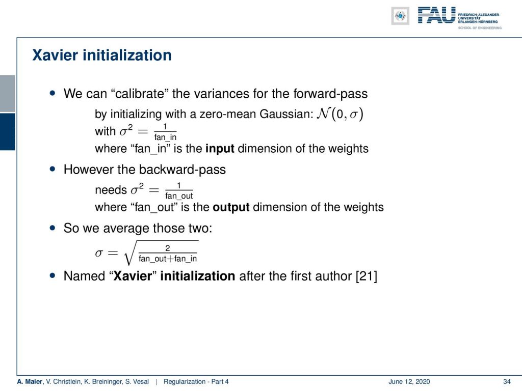
As a result, we then can work with Xavier initialization. So, we calibrate the variances for the forward pass. We initialize with a zero-mean Gaussian and we simply set the standard deviation to one over fan_in, where fan_in is the input dimension of the weights. So, we simply scale the variance to be 1 over the number of input dimensions. In the backward pass, however, we would need the same effect backward. So, we would have to scale the standard deviation with 1 over fan_out, where fan_out is the output dimension of the weights. So, you just average those two and compute a new standard deviation. This initialization is called after the first author of [21]. Well, what else can be done?

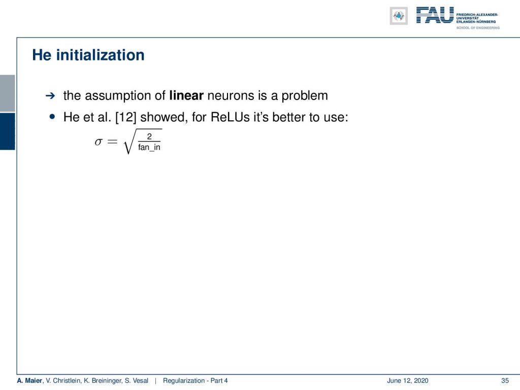
There’s He initialization which then also considers that the assumption of linear neurons is a problem. So in [12], they showed that for ReLUs, it’s better to actually use the square root of 2 over fan_in as standard deviation. So this is a very typical choice for initializing the weights randomly.

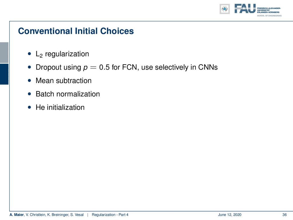
Then, other conventional initial choices are that you do L2 regularization, you use dropout with a probability of 0.5 for fully connected layers, and you use them selectively in convolutional neural networks. You do mean subtraction, batch normalization, and He initialization. So this is the very typical setup.

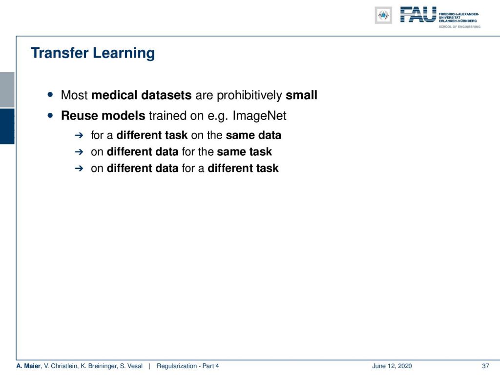
So which other tricks do we have left? One important technique is transfer learning. Now, transfer learning is typically used in all situations where you have little data. One example is medical data. There, you typically have very little data. So, the idea is then to reuse models, e.g., trained on ImageNet. You can even reuse things that have been trained on a different task for the same data. You can also use different data for the same task or you can even do different data on a different task.

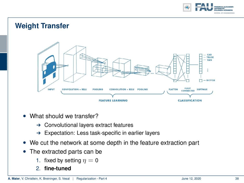
So now, the question is what should we transfer? Well, the convolutional layers extract features and the expectation now is that less task-specific features are in earlier layers. We have seen that in a couple of papers. We can also see that in our videos on visualization. So typically, those have more basic information and are likely to contain information that is worth transferring. We cut the network at some depth in the feature extraction part. For those extracted parts, we can fix the learning rate to zero. So, if we set it to zero, they won’t change. You can start fine-tuning then.

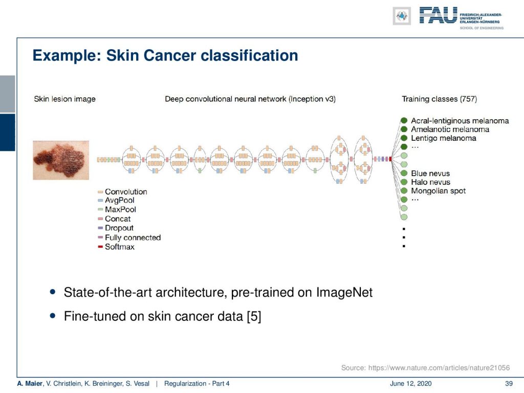
One example here is skin cancer classification. They use a deep convolutional neural network based on Inception V3. They have a state-of-the-art architecture that was pre-trained on ImageNet. Then, they fine-tune it on skin cancer data. So, they essentially take the network and what you have to replace is essentially the right-hand part. The training of the classes is something that you won’t find on ImageNet. So, there you have to replace the entire network because you want to predict very different classes. Then, you can use a couple of fully connected layers in order to map your learned feature representations to a different space. Then, you can do a classification from there.

There’s also transfer between modalities. This was also found to be beneficial. Now, you can transfer from color to x-ray and here it’s actually sufficient to simply copy the input three times. Then, you don’t need that much fine-tuning. So, this works pretty well. One alternative is that you use feature representations of other networks as a loss function. This then leads to perceptual loss. We will talk about perceptual loss in a different video. In any case transfer learning is typically a very good idea. There are many many applications and many papers where they have been using transfer learning. A long time ago, they didn’t say transfer learning but they said adaptation. In particular, in speech processing, they have speaker and noise adaptation and so on. But nowadays you say transfer learning. It’s essentially the same concept.

Next time in deep learning, we will talk about the remaining tricks of the trade and regularization. I’m looking forward to seeing you in the next lecture. So thank you very much for listening and goodbye!

If you liked this post, you can find more essays here, more educational material on Machine Learning here, or have a look at our Deep LearningLecture. I would also appreciate a clap or a follow on YouTube, Twitter, Facebook, or LinkedIn in case you want to be informed about more essays, videos, and research in the future. This article is released under the Creative Commons 4.0 Attribution License and can be reprinted and modified if referenced.

Links

Link – for details on Maximum A Posteriori estimation and the bias-variance decomposition
Link – for a comprehensive text about practical recommendations for regularization
Link – the paper about calibrating the variances

References

[1] Sergey Ioffe and Christian Szegedy. “Batch Normalization: Accelerating Deep Network Training by Reducing Internal Covariate Shift”. In: Proceedings of The 32nd International Conference on Machine Learning. 2015, pp. 448–456.
[2] Jonathan Baxter. “A Bayesian/Information Theoretic Model of Learning to Learn via Multiple Task Sampling”. In: Machine Learning 28.1 (July 1997), pp. 7–39.
[3] Christopher M. Bishop. Pattern Recognition and Machine Learning (Information Science and Statistics). Secaucus, NJ, USA: Springer-Verlag New York, Inc., 2006.
[4] Richard Caruana. “Multitask Learning: A Knowledge-Based Source of Inductive Bias”. In: Proceedings of the Tenth International Conference on Machine Learning. Morgan Kaufmann, 1993, pp. 41–48.
[5] Andre Esteva, Brett Kuprel, Roberto A Novoa, et al. “Dermatologist-level classification of skin cancer with deep neural networks”. In: Nature 542.7639 (2017), pp. 115–118.
[6] C. Ding, C. Xu, and D. Tao. “Multi-Task Pose-Invariant Face Recognition”. In: IEEE Transactions on Image Processing 24.3 (Mar. 2015), pp. 980–993.
[7] Li Wan, Matthew Zeiler, Sixin Zhang, et al. “Regularization of neural networks using drop connect”. In: Proceedings of the 30th International Conference on Machine Learning (ICML-2013), pp. 1058–1066.
[8] Nitish Srivastava, Geoffrey E Hinton, Alex Krizhevsky, et al. “Dropout: a simple way to prevent neural networks from overfitting.” In: Journal of Machine Learning Research 15.1 (2014), pp. 1929–1958.
[9] R. O. Duda, P. E. Hart, and D. G. Stork. Pattern Classification. John Wiley and Sons, inc., 2000.
[10] Ian Goodfellow, Yoshua Bengio, and Aaron Courville. Deep Learning. http://www.deeplearningbook.org. MIT Press, 2016.
[11] Yuxin Wu and Kaiming He. “Group normalization”. In: arXiv preprint arXiv:1803.08494 (2018).
[12] Kaiming He, Xiangyu Zhang, Shaoqing Ren, et al. “Delving deep into rectifiers: Surpassing human-level performance on imagenet classification”. In: Proceedings of the IEEE international conference on computer vision. 2015, pp. 1026–1034.
[13] D Ulyanov, A Vedaldi, and VS Lempitsky. Instance normalization: the missing ingredient for fast stylization. CoRR abs/1607.0 [14] Günter Klambauer, Thomas Unterthiner, Andreas Mayr, et al. “Self-Normalizing Neural Networks”. In: Advances in Neural Information Processing Systems (NIPS). Vol. abs/1706.02515. 2017. arXiv: 1706.02515.
[15] Jimmy Lei Ba, Jamie Ryan Kiros, and Geoffrey E Hinton. “Layer normalization”. In: arXiv preprint arXiv:1607.06450 (2016).
[16] Nima Tajbakhsh, Jae Y Shin, Suryakanth R Gurudu, et al. “Convolutional neural networks for medical image analysis: Full training or fine tuning?” In: IEEE transactions on medical imaging 35.5 (2016), pp. 1299–1312.
[17] Yoshua Bengio. “Practical recommendations for gradient-based training of deep architectures”. In: Neural networks: Tricks of the trade. Springer, 2012, pp. 437–478.
[18] Chiyuan Zhang, Samy Bengio, Moritz Hardt, et al. “Understanding deep learning requires rethinking generalization”. In: arXiv preprint arXiv:1611.03530 (2016).
[19] Shibani Santurkar, Dimitris Tsipras, Andrew Ilyas, et al. “How Does Batch Normalization Help Optimization?” In: arXiv e-prints, arXiv:1805.11604 (May 2018), arXiv:1805.11604. arXiv: 1805.11604 [stat.ML].
[20] Tim Salimans and Diederik P Kingma. “Weight Normalization: A Simple Reparameterization to Accelerate Training of Deep Neural Networks”. In: Advances in Neural Information Processing Systems 29. Curran Associates, Inc., 2016, pp. 901–909.
[21] Xavier Glorot and Yoshua Bengio. “Understanding the difficulty of training deep feedforward neural networks”. In: Proceedings of the Thirteenth International Conference on Artificial Intelligence 2010, pp. 249–256.
[22] Zhanpeng Zhang, Ping Luo, Chen Change Loy, et al. “Facial Landmark Detection by Deep Multi-task Learning”. In: Computer Vision – ECCV 2014: 13th European Conference, Zurich, Switzerland, Cham: Springer International Publishing, 2014, pp. 94–108.

Category: Lecture Notes in Deep Learning