Lecture Notes in Deep Learning: Common Practices – Part 1

Optimizers & Learning Rates

These are the lecture notes for FAU’s YouTube Lecture “Deep Learning“. This is a full transcript of the lecture video & matching slides. We hope, you enjoy this as much as the videos. Of course, this transcript was created with deep learning techniques largely automatically and only minor manual modifications were performed. If you spot mistakes, please let us know!

Welcome everybody to today’s deep learning lecture! Today, we want to talk a bit about common practices. The stuff that you need to know to get everything implemented in practice,

So, I have a small outline over the next couple of videos and the topics that we will look at. So, we will think about the problems that we currently have and how far we went. We will talk about training strategies, again optimization and learning rates, and a couple of tricks on how to adjust them, architecture selection, and hyperparameter optimization. One trick that is really useful is ensembling. Typically people have to deal with the class imbalance and of course, there are also very interesting approaches to deal with this. So finally, we look into the evaluation and how to get a good predictor. We also estimate how well our network is actually performing.

So far, we have seen all the nuts and bolts of how to train the network. We have to fully connected and convolutional layers, the activation function, the loss function, optimization, regularization, and today we will talk about how to choose the architecture, train, and evaluate a deep neural network.

The very first thing is testing. “Ideally, the test data should be kept in a vault and be brought only out at the end of the data analysis.” as Hastie and colleagues are teaching in the elements of statistical learning.

So, first things first: Overfitting is extremely easy with neural networks. Remember the ImageNet random labels. The true test set error and generalization can be underestimated substantially when you use the test set for model selection. So, when we choose the architecture – typically the first element in the model selection – this should never be done on the test set. We can do initial experimentation on a smaller subset of the data to try to figure out what works. Never work on the test set when you’re doing these things.

Let’s look at a couple of training strategies: Before the training check your gradients, check the loss function, check own layer implementations that they compute results correctly. If you implemented your own layer, then compare the analytic and the numeric gradient. You can use central differences for the numeric gradient. You can use relative errors instead of absolute differences and consider the numerics. Use double precision for checking, temporally scale the loss function, and if you observe very small values, choose your h for the step size appropriately.

Then, we have a couple of additional and recommendations: If you only use a few data points, then you will have fewer issues with non-differentiable parts of the loss function. You can train the network for a short period of time and only then perform the gradient checks. You can check the gradient first, then with regularization terms. So, you first turn the regularization terms off, check the gradient, and in the end with the regularization terms. Also, turn off data augmentation and drop out. So, you typically make this check on rather small data sets.

The goal of the initialization is that you have a correct random initialization of the layers. So, you can compute the loss for each class on the untrained network with regularization turned off and of course, that should give a random classification. So here, one can compare the loss with the loss achieved when deciding for class randomly. They should be the same because you randomly initialize. Repeat this with multiple random initializations just to check that there’s nothing wrong with the initialization.

Let’s go to training. First, you check whether the architecture is in general capable of learning the task. So, before training the network on the full data set, you take a small subset of the data. Maybe five to 20 samples and then try to overfit the network to get a zero loss. With such few samples, you should be able to memorize the entire data set. Try to get a zero loss. Then, you know that your training procedure actually works and you can really go down to the zero loss. Optionally, you can turn off the regularization because it may hinder this overfitting procedure. Now, if the network can’t overfit, you may have a bug in the implementation, or your model may be too small. So, you may want to increase the parameters / the model capacity or simply the model may not be suitable for this task. Also, get a first idea about how the data, the loss, and the network behave.

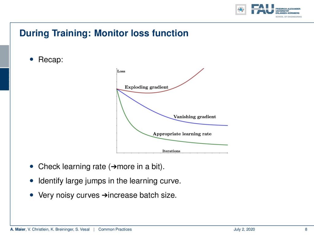
Remember, we should monitor the loss function. These are typical loss curves. Make sure you don’t have an exploding or vanishing gradient. You want to have the appropriate learning rate, so check the learning rate to identify large jumps in the learning curve. If you have very noisy curves, try to increase the batch size. Noisy loss curves can be associated with too small mini-batches.

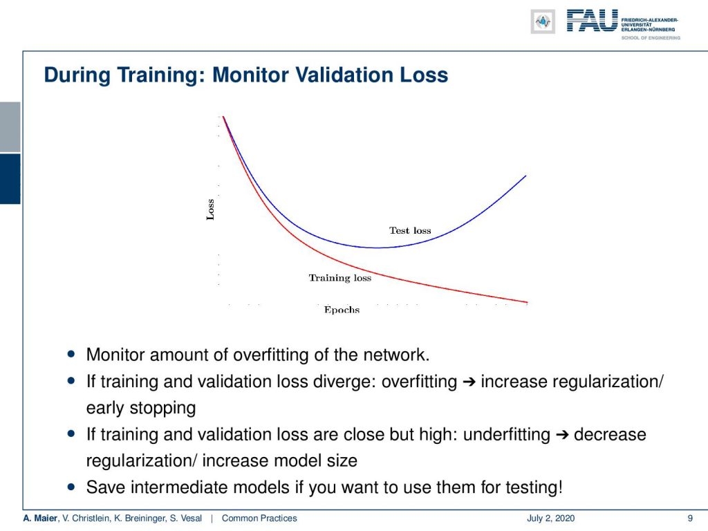
Next, get a validation data set and monitor the validation loss. You remember, this image here: Over the epochs, your training loss will, of course, go down but the test loss would go up. You never compute, of course, this on the test data set but you take the validation set as a surrogate for the test loss. Then, you can identify whether overfitting occurs in your network. If training and validation diverge, you have overfitting. So, you may want to increase the regularization or try early stopping. If training and validation loss are close but very high, you may have underfitting. So, decrease the regularization and increase the model size. You may want to save intermediate models because you can use them for testing later.

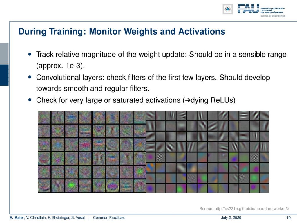
Further, during training monitor the weights and the activations. Keep track of the relative magnitude of the weight update. They should be in a sensible range, maybe 10⁻³. In the convolutional layers, you can check the filters of the first few layers. They should develop towards smooth and regular filters. You may want to check that. You want to get filters like here, on the right-hand side. The ones on the left-hand side, contain considerable amounts of noise and this may be not very reliable features. You may start building a noise detector here. So this can be a problem. Also, check for largely saturated activations. Keep in mind that dying ReLUs may happen.

So let’s look a bit at optimization and the learning rate. You want to choose an optimizer. Now, batch gradient descent requires large memory, is too slow, and has too few updates. So what people go for is typically stochastic gradient descent. Here, the loss function and the gradient become very noisy, in particular, if you only use one of your samples. You want to go with the mini-batch. The mini-batch is the best of both worlds. It has frequent but stable updates and the gradient is noisy enough to escape local minima. So, you want to adapt the mini-batch size to yield smoother or more noisy gradients, depending on your problem and the optimization. In addition, you may want to use momentum to prevent oscillations and speed up the optimization. The effect of hyper-parameters is relatively straightforward. The recommendation from us is you start with mini-batch, gradient descent, and momentum. Once, you have a good parameter set, you then change to Adam or other optimizers that can optimize the different weights with an adaptive learning rate.

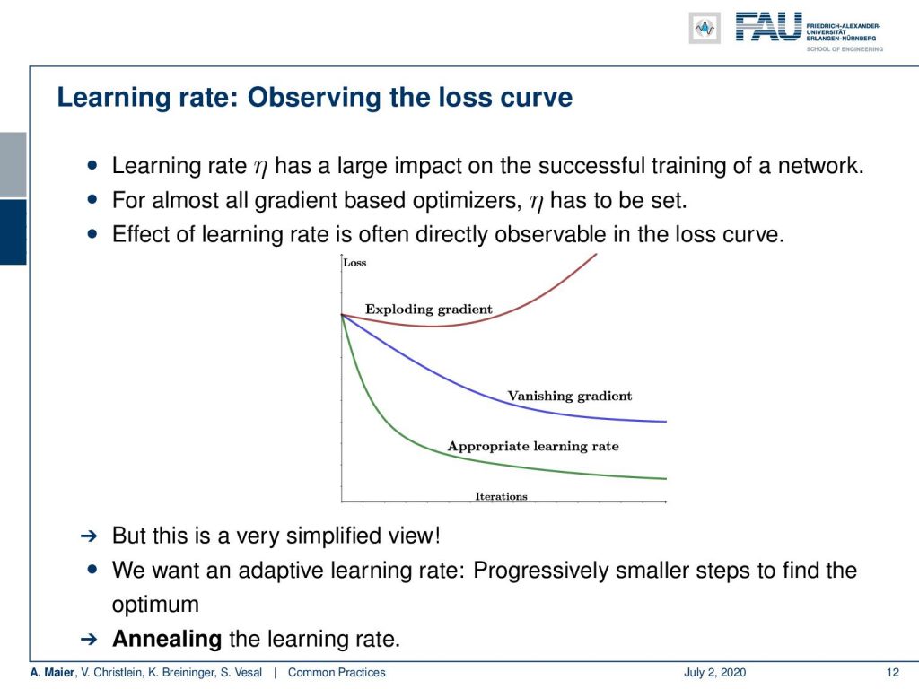
Keep in mind to observe the loss curve. If your learning rate is not set correctly, you have trouble in the training of the network. For almost all gradient-based optimizers, you have to set η. So, we often see that directly in the lost curve, but this is a simplified view. So we actually want to have an adaptive learning rate and then progressively have smaller steps to find the optimum. So as we already discussed, you want to anneal the learning rate.

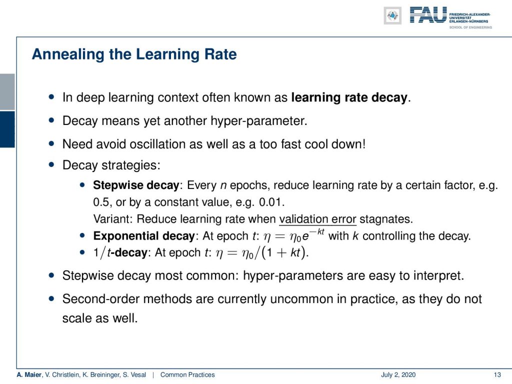
Now, the learning rate decay is yet another hyper-parameter that you have to set somehow. You want to avoid oscillations as well as a too-fast cooldown. So, there’s a couple of decay strategies. Stepwise decay every n epochs, you reduce the learning rate by a certain factor, like 0.5, a constant value like 0.01, or you reduce the learning rate when the validation error is no longer reducing. There’s exponential decay at every epoch where you actually use this exponential function here that can control the decay. There’s also the 1/t decay that at epoch t, you essentially scale the initial learning rate with 1 / (1 + kt). The stepwise decay is most common and also the hyper-parameters are easy to interpret. Second-order methods are currently uncommon in practice as they don’t scale very well. So much about learning rates and a couple of the associated hyper-parameters.

Next time in deep learning, we will look further into how to adjust all those hyper-parameters that we’ve just discovered. You will find those hints to be really valuable for your own experimentation. So thank you very much for listening and see you in the next lecture!

If you liked this post, you can find more essays here, more educational material on Machine Learning here, or have a look at our Deep LearningLecture. I would also appreciate a follow on YouTube, Twitter, Facebook, or LinkedIn in case you want to be informed about more essays, videos, and research in the future. This article is released under the Creative Commons 4.0 Attribution License and can be reprinted and modified if referenced.

References

[1] M. Aubreville, M. Krappmann, C. Bertram, et al. “A Guided Spatial Transformer Network for Histology Cell Differentiation”. In: ArXiv e-prints (July 2017). arXiv: 1707.08525 [cs.CV].
[2] James Bergstra and Yoshua Bengio. “Random Search for Hyper-parameter Optimization”. In: J. Mach. Learn. Res. 13 (Feb. 2012), pp. 281–305.
[3] Jean Dickinson Gibbons and Subhabrata Chakraborti. “Nonparametric statistical inference”. In: International encyclopedia of statistical science. Springer, 2011, pp. 977–979.
[4] Yoshua Bengio. “Practical recommendations for gradient-based training of deep architectures”. In: Neural networks: Tricks of the trade. Springer, 2012, pp. 437–478.
[5] Chiyuan Zhang, Samy Bengio, Moritz Hardt, et al. “Understanding deep learning requires rethinking generalization”. In: arXiv preprint arXiv:1611.03530 (2016).
[6] Boris T Polyak and Anatoli B Juditsky. “Acceleration of stochastic approximation by averaging”. In: SIAM Journal on Control and Optimization 30.4 (1992), pp. 838–855.
[7] Prajit Ramachandran, Barret Zoph, and Quoc V. Le. “Searching for Activation Functions”. In: CoRR abs/1710.05941 (2017). arXiv: 1710.05941.
[8] Stefan Steidl, Michael Levit, Anton Batliner, et al. “Of All Things the Measure is Man: Automatic Classification of Emotions and Inter-labeler Consistency”. In: Proc. of ICASSP. IEEE – Institute of Electrical and Electronics Engineers, Mar. 2005.

Category: Lecture Notes in Deep Learning