Lecture Notes in Deep Learning: Architectures – Part 2

Deeper Architectures

These are the lecture notes for FAU’s YouTube Lecture “Deep Learning“. This is a full transcript of the lecture video & matching slides. We hope, you enjoy this as much as the videos. Of course, this transcript was created with deep learning techniques largely automatically and only minor manual modifications were performed. If you spot mistakes, please let us know!

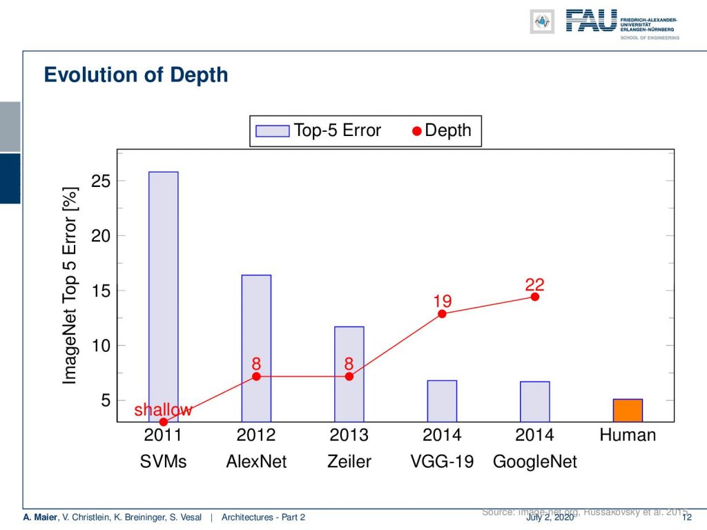
Welcome back to deep learning! Today I want to talk about part two of the architectures. Now, we want to go even a bit deeper in the second part: Deeper models. So, we see that going deeper really was very beneficial for the error rate. So, you can see the results on ImageNet here. In 2011, with a shallow support vector machine, you see that the error rates were really high with 25%. AlexNet already almost cut it to half in 2012. Then Zeiler in 2013, was the next winner with again eight layers. VGG in 2014: 19 layers. GoogleNet in 2014: 22 layers, also almost the same performance. So, you can see that the more we increase the depth, the better seemingly the performance gets. We can see there’s only a little bit of margin left in order to beat human performance.

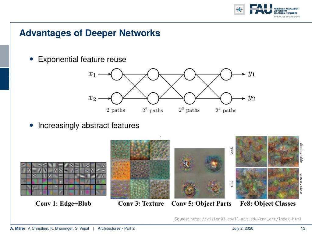
Depth seems to play a key role in building good networks. Why could that be the case? One reason why those deeper networks may be very efficient is something that we call exponential feature reuse. So here you can see if we only had two features. If we stack neurons on top, you can see that the number of possible paths is exponentially increasing. So with two neurons, I have two paths. With another layer of neurons, I have 2² paths. With three layers 2³ paths, 2⁴ paths, and so on. So deeper networks seem somehow to be able to reuse information from the previous layers. We can also see that if we look at what they are doing. If we generate get these visualizations, we see that they increasingly build more abstract representations. So, we somehow see a kind of modularization happening. We think that deep learning works because we are able to have different parts of the function at different positions. So we are disentangling somehow the processing into simpler steps and then we essentially train a program with multiple steps that is able to describe more and more abstract representations. So here we see the first layers, they do maybe edges and blobs. Let’s say, layer number three detects those textures. Layer number five perceives object parts, and layer number eight already object classes. These images here are created from visualizations from AlexNet. So you can see that this somehow seems to be happening really in the network. This is also probably a key reason why deep learning works. We are able to disentangle the function as we try to compute different things at different positions.

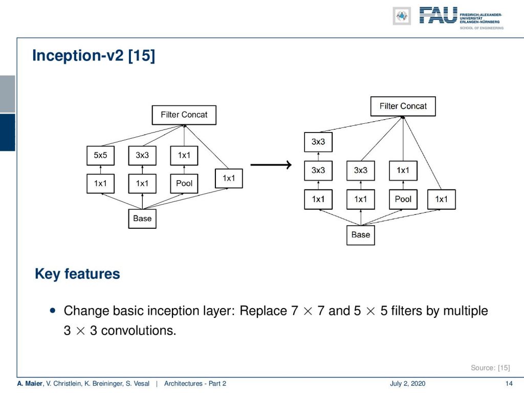
Well, we want to go deeper and one technology that has been implemented there is again the inception modules. The improved Inception modules now essentially replace those filters that we’ve seen with the 5×5 convolutions and 3×3 convolutions into multiple of those conclusions. Instead of doing a 5×5 convolution, you do two 3×3 convolutions in a row. That already saves a couple of computations and you can then replace 5×5 filters by stacking filters on top. We can see that this actually works for a broad variety of kernels that you can actually separate into several steps after another. So, you can cascade them. This filter cascading is something that you would also discuss in a typical computer vision class.

So Inception V2 then already had 42 layers. They start with essentially 3×3 convolutions and three modified inception modules like the one that we just looked at. Then in the next layer, an efficient grid size reduction is introduced that is using strided convolutions. So, you have 1×1 convolutions for channel compression, 3×3 convolutions with stride 1 followed by a 3×3 convolution with a stride of 2. This essentially effectively replaces the different pooling operations. The next idea then was to five times introduce modules of flattened convolutions. Here the idea is to express the convolutions no longer in 2-D convolutions but instead, you separate them into convolutions in x and y-direction. You alternatingly produce those 2 convolutions. So you can see here, we start with 1×1 convolutions in the left branch. Then we do a 1xn convolution followed by a nx1 convolution, followed by a 1xn convolution and so on. This allows us essentially to break down kernels into two directions. So, you know because you alternatingly change the orientation of the convolution, you are essentially breaking up the 2-D convolutions by forced separable computation. We can also see that separation of convolution filters works for a broad variety of filters. Of course, this is a restriction as it doesn’t allow all of the possible computations. But remember, we have in the earlier layers full 3×3 convolutions. So they can already learn how to adopt for the later layers. As a result, they can then be processed by the separable convolutions.

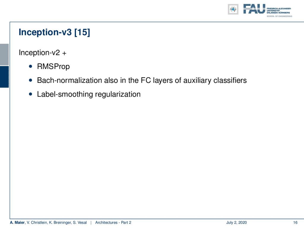
This then leads to Inception V3. For the third version of Inception, they used essentially Inception V2 and introduced RMSprop for the training procedure, batch normalization also in the fully connected layers of the auxiliary classifiers, and label smoothing regularization.

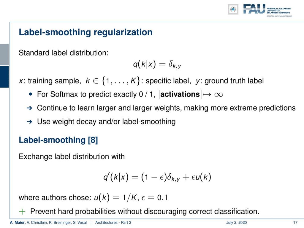
Label smoothing regularization is a really cool trick. So let’s spend a couple of more minutes looking into that idea. Now, if you think about how our label vectors typically look like, we have one hot encoded vectors. This means that our label is essentially a Dirac distribution. This essentially says that one element is correct and all others are wrong. We typically use a softmax. So this means that our activations have a tendency to go towards infinity. This is not so great because we continue to learn larger and larger weights making them more and more extreme. So, we can prevent that if we use weight decay. This will prevent our weights from growing dramatically. We can also use in addition label smoothing. The idea of label smoothing is that instead of using only the Dirac pulse, we kind of smear the probability mass onto the other classes. This is very helpful, in particular, in things like ImageNet where you have rather noisy labels. So, you remember the cases that were not entirely clear. In these noisy label cases, you can see that this label smoothing can really help. The idea is that you multiply your Dirac distribution with one minus some small number ϵ. You then distribute the ϵ that you deducted from the correct class to all the other classes in an equal distribution. So you can see here that is simply 1/K where K is the number of classes. The nice thing about this label smoothing is that you essentially discourage very hard decisions. This really helps in the case of noisy labels. So this is a very nice trick that can help you with building deeper models.

Next time, we want to look into building those really deep models. With what we have seen so far, we would ask: Why not just stack more and layers on top? Well, there’s a couple of problems that emerge if you try to do that and we will look into the reasons for that in the next video. We will also propose some solutions to going really deep. So, thank you very much for listening and see you in the next video.

If you liked this post, you can find more essays here, more educational material on Machine Learning here, or have a look at our Deep LearningLecture. I would also appreciate a follow on YouTube, Twitter, Facebook, or LinkedIn in case you want to be informed about more essays, videos, and research in the future. This article is released under the Creative Commons 4.0 Attribution License and can be reprinted and modified if referenced.

References

[1] Klaus Greff, Rupesh K. Srivastava, and Jürgen Schmidhuber. “Highway and Residual Networks learn Unrolled Iterative Estimation”. In: International Conference on Learning Representations (ICLR). Toulon, Apr. 2017. arXiv: 1612.07771.
[2] Kaiming He, Xiangyu Zhang, Shaoqing Ren, et al. “Deep Residual Learning for Image Recognition”. In: 2016 IEEE Conference on Computer Vision and Pattern Recognition (CVPR). Las Vegas, June 2016, pp. 770–778. arXiv: 1512.03385.
[3] Kaiming He, Xiangyu Zhang, Shaoqing Ren, et al. “Identity mappings in deep residual networks”. In: Computer Vision – ECCV 2016: 14th European Conference, Amsterdam, The Netherlands, 2016, pp. 630–645. arXiv: 1603.05027.
[4] J. Hu, L. Shen, and G. Sun. “Squeeze-and-Excitation Networks”. In: ArXiv e-prints (Sept. 2017). arXiv: 1709.01507 [cs.CV].
[5] Gao Huang, Yu Sun, Zhuang Liu, et al. “Deep Networks with Stochastic Depth”. In: Computer Vision – ECCV 2016, Proceedings, Part IV. Cham: Springer International Publishing, 2016, pp. 646–661.
[6] Gao Huang, Zhuang Liu, and Kilian Q. Weinberger. “Densely Connected Convolutional Networks”. In: 2017 IEEE Conference on Computer Vision and Pattern Recognition (CVPR). Honolulu, July 2017. arXiv: 1608.06993.
[7] Alex Krizhevsky, Ilya Sutskever, and Geoffrey E Hinton. “ImageNet Classification with Deep Convolutional Neural Networks”. In: Advances In Neural Information Processing Systems 25. Curran Associates, Inc., 2012, pp. 1097–1105. arXiv: 1102.0183.
[8] Yann A LeCun, Léon Bottou, Genevieve B Orr, et al. “Efficient BackProp”. In: Neural Networks: Tricks of the Trade: Second Edition. Vol. 75. Berlin, Heidelberg: Springer Berlin Heidelberg, 2012, pp. 9–48.
[9] Y LeCun, L Bottou, Y Bengio, et al. “Gradient-based Learning Applied to Document Recognition”. In: Proceedings of the IEEE 86.11 (Nov. 1998), pp. 2278–2324. arXiv: 1102.0183.
[10] Min Lin, Qiang Chen, and Shuicheng Yan. “Network in network”. In: International Conference on Learning Representations. Banff, Canada, Apr. 2014. arXiv: 1102.0183.
[11] Olga Russakovsky, Jia Deng, Hao Su, et al. “ImageNet Large Scale Visual Recognition Challenge”. In: International Journal of Computer Vision 115.3 (Dec. 2015), pp. 211–252.
[12] Karen Simonyan and Andrew Zisserman. “Very Deep Convolutional Networks for Large-Scale Image Recognition”. In: International Conference on Learning Representations (ICLR). San Diego, May 2015. arXiv: 1409.1556.
[13] Rupesh Kumar Srivastava, Klaus Greff, Urgen Schmidhuber, et al. “Training Very Deep Networks”. In: Advances in Neural Information Processing Systems 28. Curran Associates, Inc., 2015, pp. 2377–2385. arXiv: 1507.06228.
[14] C. Szegedy, Wei Liu, Yangqing Jia, et al. “Going deeper with convolutions”. In: 2015 IEEE Conference on Computer Vision and Pattern Recognition (CVPR). June 2015, pp. 1–9.
[15] C. Szegedy, V. Vanhoucke, S. Ioffe, et al. “Rethinking the Inception Architecture for Computer Vision”. In: 2016 IEEE Conference on Computer Vision and Pattern Recognition (CVPR). June 2016, pp. 2818–2826.
[16] Christian Szegedy, Sergey Ioffe, and Vincent Vanhoucke. “Inception-v4, Inception-ResNet and the Impact of Residual Connections on Learning”. In: Thirty-First AAAI Conference on Artificial Intelligence (AAAI-17) Inception-v4, San Francisco, Feb. 2017. arXiv: 1602.07261.
[17] Andreas Veit, Michael J Wilber, and Serge Belongie. “Residual Networks Behave Like Ensembles of Relatively Shallow Networks”. In: Advances in Neural Information Processing Systems 29. Curran Associates, Inc., 2016, pp. 550–558. A.
[18] Di Xie, Jiang Xiong, and Shiliang Pu. “All You Need is Beyond a Good Init: Exploring Better Solution for Training Extremely Deep Convolutional Neural Networks with Orthonormality and Modulation”. In: 2017 IEEE Conference on Computer Vision and Pattern Recognition (CVPR). Honolulu, July 2017. arXiv: 1703.01827.
[19] Lingxi Xie and Alan Yuille. Genetic CNN. Tech. rep. 2017. arXiv: 1703.01513.
[20] Sergey Zagoruyko and Nikos Komodakis. “Wide Residual Networks”. In: Proceedings of the British Machine Vision Conference (BMVC). BMVA Press, Sept. 2016, pp. 87.1–87.12.
[21] K Zhang, M Sun, X Han, et al. “Residual Networks of Residual Networks: Multilevel Residual Networks”. In: IEEE Transactions on Circuits and Systems for Video Technology PP.99 (2017), p. 1.
[22] Barret Zoph, Vijay Vasudevan, Jonathon Shlens, et al. Learning Transferable Architectures for Scalable

Category: Lecture Notes in Deep Learning