
From LeNet to GoogLeNet
These are the lecture notes for FAU’s YouTube Lecture “Deep Learning“. This is a full transcript of the lecture video & matching slides. We hope, you enjoy this as much as the videos. Of course, this transcript was created with deep learning techniques largely automatically and only minor manual modifications were performed. If you spot mistakes, please let us know!
Welcome back to deep learning and you can see in the video, I have a couple of upgrades. We have a much better recording quality now and I hope you can also see that I finally fixed the sound problem. You should be able to hear me much better right now. We are back for a new session and we want to talk about a couple of exciting topics. So, let’s see what I’ve got for you. So today I want to start discussing different architectures. In particular, in the first couple of videos, I want to talk a bit about the early architectures. the things that we’ve seen in the very early days of deep learning. We will follow then by looking into deeper models in later videos and in the end we want to talk about learning architectures.

A lot of what we’ll see in the next couple of slides and videos have of course being developed for image recognition and object detection tasks. In particular two data sets are very important for these kinds of tasks. This is the ImageNet data set which you find in [11]. It has something like a thousand classes and more than 14 million images. Subsets have been used for the ImageNet large-scale visual recognition challenges. It contains natural images of varying sizes. So, a lot of these images have actually been downloaded from the internet. There are also smaller data sets if you don’t want to train with like millions of images right away. So, they are also very important. CIFAR 10 and CIFAR 100 have 10 and 100 classes respectively. In both, we only have 50k training and 10k testing images. The images have reduced size: 32 x 32 in order to very quickly be able to explore different architectures. If you have these smaller data sets then it also doesn’t take so long for training. So this is also a very common data set if you want to evaluate your architecture.
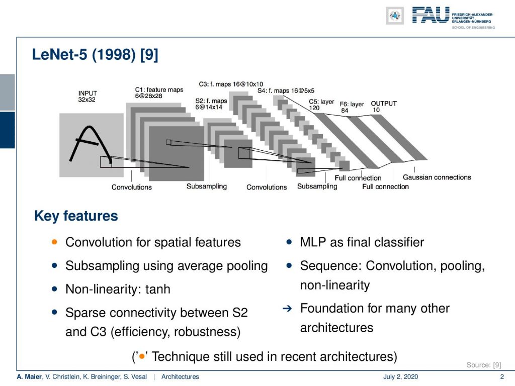
Based on these different data sets, we then want to go ahead and look into the early architectures. I think one of the most important ones is LeNet which was published in 1998 in [9]. You can see this is essentially the convolutional neural network (CNN) that we have been discussing so far. It has been used for example for letter recognition. We have the convolutional layers that have trainable kernels and pooling, another set of convolutional layers, and another pooling operation, and then towards the end, we are going into fully connected layers. Hence, we gradually reduce dimensionality and at the very end, we have the output layer that corresponds to the number of classes. This is a very typical CNN type of architecture and this kind of approach has been used in many papers. This has inspired a lot of work. We have for every architecture here key features and you can see, here, most of the bullets are in gray. That means that most of these features did not survive. Of course, what survived here was convolution for spatial features. This is the main idea that is still prevalent. All the other things like subsampling using average pooling did not take the test of time. It still used as non-linearity the hyperbolic tangent. So, it’s a not-so-deep model, right? Then, it had sparse connectivity between S2 and C3 layers, as you see here in the figure. So also not that common anymore is the multi-layer perceptron as the final classifier. This is something that we see no longer because it has been replaced by for example fully convolutional networks. This is a much more flexible approach and also the sequence of convolution pooling and non-linearity is kind of fixed. Today, we will do that in a much better way but of course, this architecture is fundamental for many of the further developments. So, I think it’s really important that we are also listing it here.
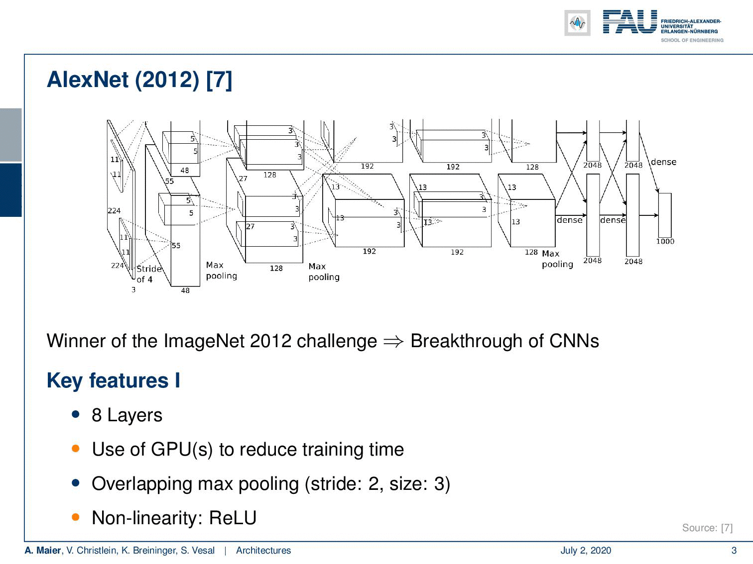
The next milestone that I want to talk about in this video is AlexNet. You find the typical image here. By the way, you will find exactly this image also in the original publication. So, Alex net is consisting of those two branches that you see here and you can see that even in the original publication, the top branch is cut in half. So, it’s a kind of artifact that you find in many representations of AlexNet when they refer to this figure. So, the figure is cut into parts but it’s not that severe because those two parts are essentially identical. One of the reasons why it was split into two sub-networks, you could say is because AlexNet has been implemented on graphical processing units (GPUs). So this is implemented on GPUs and it actually was already multi-GPU. So, the two branches that you see on the top, have been implemented on two different graphics processing units and they could also be trained and then synchronized using the software. So, the GPU is of course a feature that is still very prevalent. You know everybody today in deep learning is very much relying on graphic processing units. As we’ve seen on numerous occasions in this lecture, it had essentially eight layers. So it’s not such a deep network. It had overlapping max pooling with a stride of two and a size of three. It introduced the ReLU non-linearity which is also very very commonly used today. So this is also a very important feature. Of course, it is the winner of the 2012 ImageNet challenge which essentially cut down the error rate into half. So it’s really one of the milestones towards the breakthrough of CNN’s. What else do we have? To combat overfitting in this architecture already dropout with a probability of 0.5 was used in the first two fully connected layers. Also, data augmentation was included. So there were random transformations and random intensity variations. Another key feature was that it has been employing mini-batch stochastic gradient descent with momentum 0.9 and an L2 weight decay with a parameter setting of 5 times 10⁻⁵. It was using a rather simple weight initialization. Just using a normal distribution and a small standard deviation. In previous lectures, we have seen much better approaches. What else is important? Well, we’ve seen that GPU separation has a historical reason. The GPUs at the time were too small to host the entire network, so it was split into two GPUs.
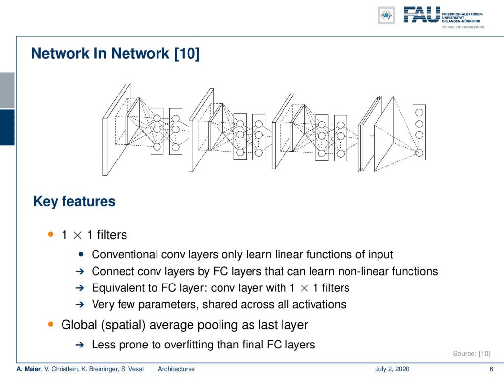
Another key paper, I would say is the Network-in-Network paper where they essentially introduced 1×1 filters. This was originally described as a network in a network but effectively we know it today as 1×1 convolutions because they essentially introduced fully connected layers over the channels. We use this recipe now a lot if you want to compress channels as we fully connect over the channel dimension. So, this is very nice because we’ve seen already that this is equivalent to a fully connected layer. We can now integrate fully connected layers in terms of 1×1 convolution and this enables us this very nice concept of the fully convolutional networks. So it has very few parameters shared across all the activations. Using global spatial average pooling as the last layer, this is essentially the birth of fully convolutional neural networks.
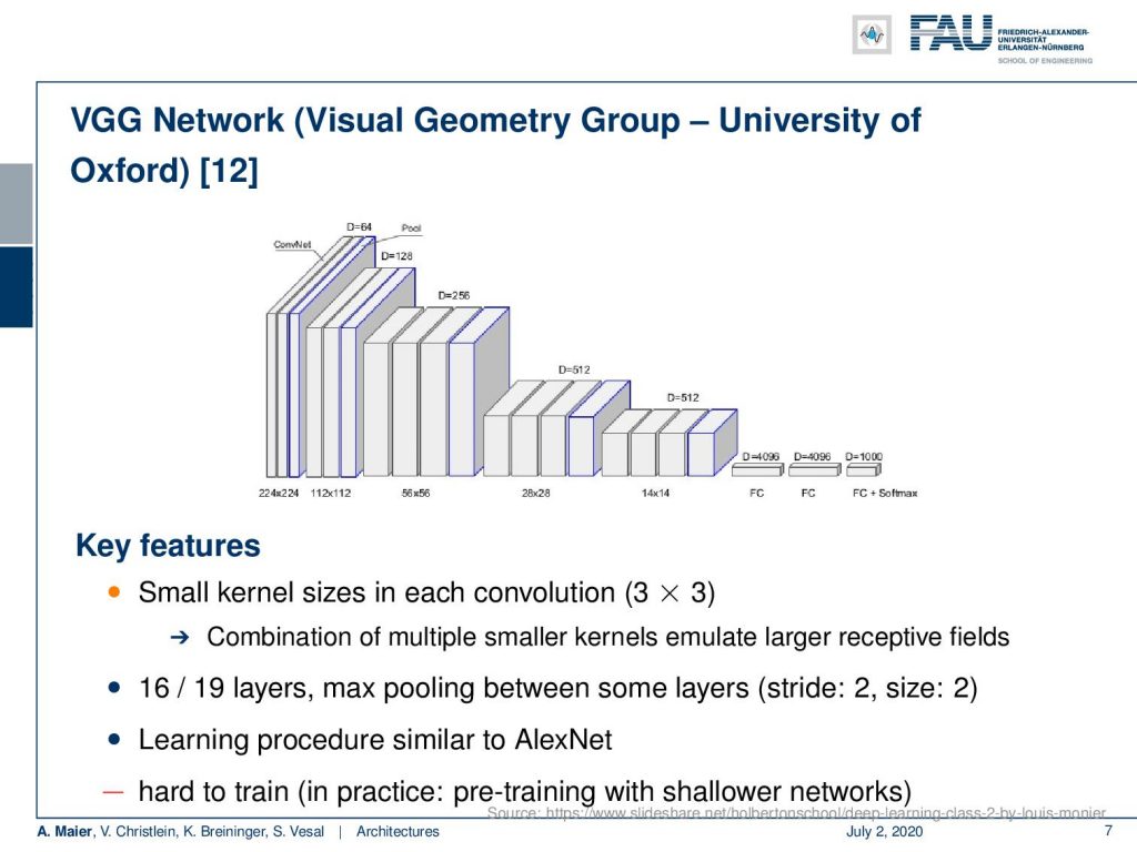
Another very important architecture is the VGG network of the Visual Geometry Group (VGG) of the University of Oxford. They introduced small kernel sizes in each convolution. The network is also very common because it’s available for download. So, there are pre-trained models available and you can see that the key feature that they have in this network is that they essentially reduce the spatial dimension as they increase the channel dimension step by step. This is a gradual transformation from the spatial domain into a let’s say for the classifier important interpretation domain. So, we can see the spatial dimension goes down and at the same time we go up with the channel dimension. This allows us to gradually convert from color images towards meaning. So, I think the small kernel size is the key feature that is still used. It was typically used in 16 and 19 layers with max-pooling between some of the layers. The learning procedure was very similar to AlexNet but turned out to be hard to train. In practice, you needed pre-training with shallower networks in order to construct this. So the network is not so great in terms of performance and has a lot of parameters but it’s pre-trained and it’s available. Therefore this has also caused the community to adopt this quite widely. So, you can see also when you work with open source and accessible software, this is also a key feature that is important for others in order to develop further concepts. Parameters can be shared. Trained models can be shared. Source code can be shared. This is why I think this is a very important instance in the deep learning landscape.
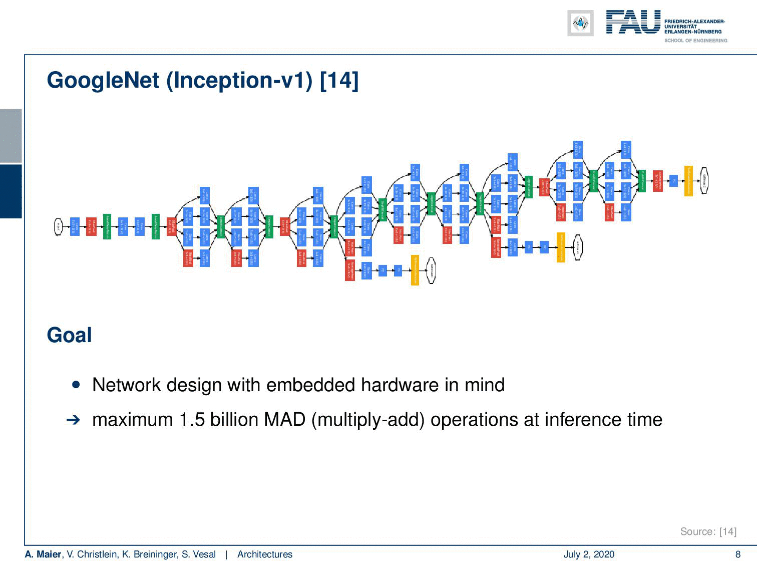
Another key network that we already seen on quite some occasions in this lecture is GoogleNet. Here, we have the inception V1 version that you find in [14]. I think the main points that I want to highlight here are that they had very good ideas in order to save computations by using a couple of tricks. So, they developed these networks with embedded hardware in mind and it also just features 1.5 billion multiply-add operations (MAD) in the inference time. This is pretty cool but what I find even cooler are these inception blocks. So in total, it had 22 layers and the global average pooling as a final layer. These inception modules are really nice and we will look at them in a little more detail on the next slide because they essentially allow you to let the network decide whether it wants to pool or whether it wants to convolve. This is pretty cool. Another trick that is really nice is using these auxiliary classifiers that they apply in earlier layers in order to stabilize the gradient. So, the idea is that you plug in your loss into some of the more early layers where you already try to figure out a preliminary classification. This helps to build deeper models because you can bring in the loss at a rather early stage. You know the deeper you go into the network, the more you go to the earlier layers, the more likely it is that you get a vanishing gradient. With these auxiliary classifiers, you can prevent it to some extent. It’s also quite useful if you, for example, want to figure out how many of those inceptions modules do you really need. Then, you can work with those axillary classifiers. So that’s really a very interesting concept.
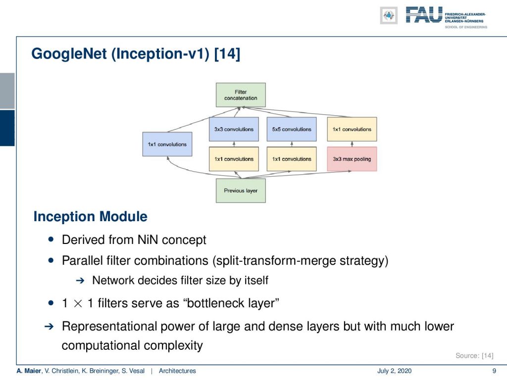
So let’s talk a bit about those inception modules. By the way, the inception modules are of course something that has survived for quite some time and it’s still being used in many of the state-of-the-art deep learning models. So there are different branches through these networks. There’s like only a 1×1 convolution, a 1×1 convolution followed by a 3×3 convolution, or 1×1 convolution followed by a 5×5 convolution or max-pooling followed by 1×1 convolution. So all of these branches go in parallel and then you concatenate the output of the branches and offer it to the next layer. So, essentially this allows then the network to decide which of the branches it trusts in the next layer. This way it can somehow determine whether it wants to pool or whether it wants to convolve. So, you can essentially think about this as an automatic routing that is determined during the training.
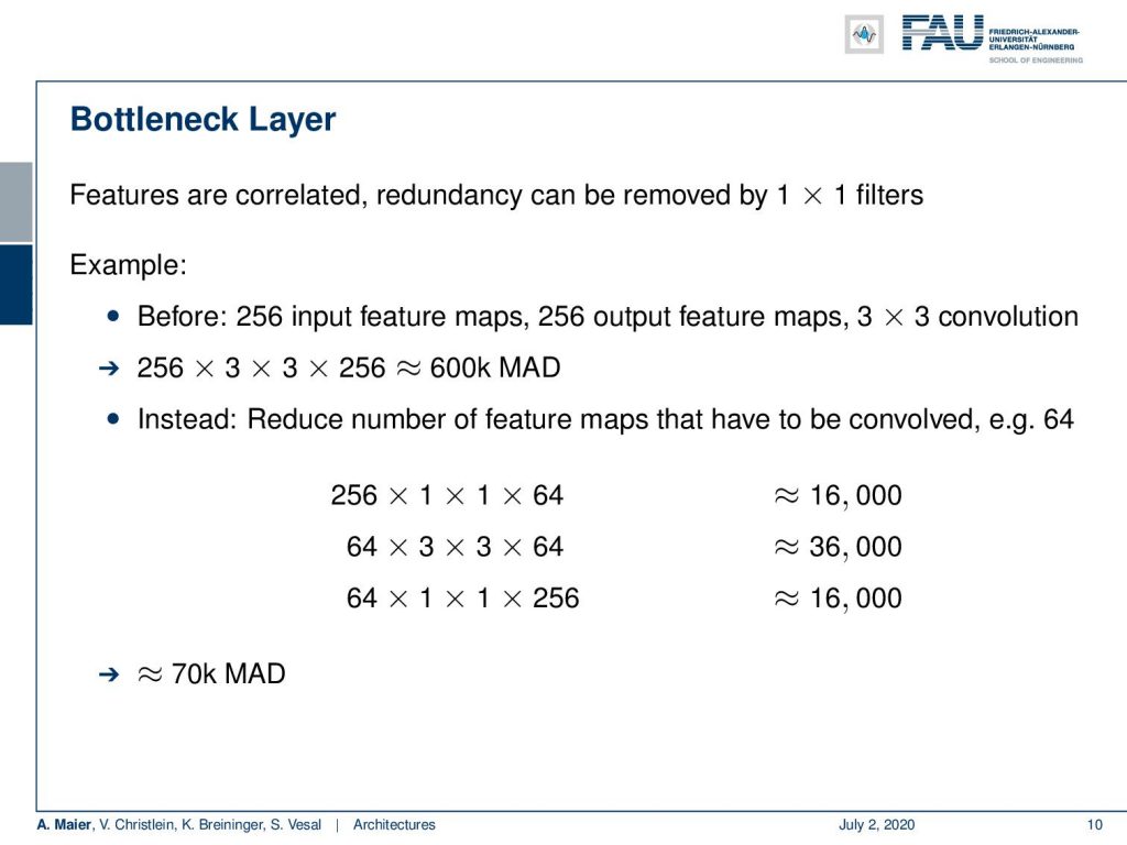
Also interesting is that the 1×1 filters serve as a kind of bottleneck layer. So, you can use that in order to compress the channels from the previous layers. Then, you can compress and then convolve. Still, there’s a lot of computations if you were to implement it exactly this way. So, the idea is then that they use this bottleneck layer in order to essentially compress the correlations between different feature maps. The idea is that you have these 1×1 filters. What you do is omit additional computations. Let’s say you route 256 input feature maps and 256 output feature maps through a 3×3 convolution, this would already mean that you have something like 600,000 multiply-add operations. So instead, you use these bottleneck ideas. You compress the channels from 256 by 1×1 convolution to 64. Then you do on the 64 channels the 3×3 convolution. Next, you uncompress essentially from the 64 channels again to 256. This saves a lot of computations. In total, you need approximately 70.000 multiply-add operations. If you look at the original 600,000 multiply-add operations, then you can see that we already saved a lot of computing operations.
Okay, so these are essentially classical deep learning architectures. We want to talk about more sophisticated ones in the second part and there I want to show you how to go even deeper and how you can do that efficiently with for example other versions of the inception module. So thank you very much for listening and hope to see you in the next video goodbye!
If you liked this post, you can find more essays here, more educational material on Machine Learning here, or have a look at our Deep LearningLecture. I would also appreciate a follow on YouTube, Twitter, Facebook, or LinkedIn in case you want to be informed about more essays, videos, and research in the future. This article is released under the Creative Commons 4.0 Attribution License and can be reprinted and modified if referenced.
References
[1] Klaus Greff, Rupesh K. Srivastava, and Jürgen Schmidhuber. “Highway and Residual Networks learn Unrolled Iterative Estimation”. In: International Conference on Learning Representations (ICLR). Toulon, Apr. 2017. arXiv: 1612.07771.
[2] Kaiming He, Xiangyu Zhang, Shaoqing Ren, et al. “Deep Residual Learning for Image Recognition”. In: 2016 IEEE Conference on Computer Vision and Pattern Recognition (CVPR). Las Vegas, June 2016, pp. 770–778. arXiv: 1512.03385.
[3] Kaiming He, Xiangyu Zhang, Shaoqing Ren, et al. “Identity mappings in deep residual networks”. In: Computer Vision – ECCV 2016: 14th European Conference, Amsterdam, The Netherlands, 2016, pp. 630–645. arXiv: 1603.05027.
[4] J. Hu, L. Shen, and G. Sun. “Squeeze-and-Excitation Networks”. In: ArXiv e-prints (Sept. 2017). arXiv: 1709.01507 [cs.CV].
[5] Gao Huang, Yu Sun, Zhuang Liu, et al. “Deep Networks with Stochastic Depth”. In: Computer Vision – ECCV 2016, Proceedings, Part IV. Cham: Springer International Publishing, 2016, pp. 646–661.
[6] Gao Huang, Zhuang Liu, and Kilian Q. Weinberger. “Densely Connected Convolutional Networks”. In: 2017 IEEE Conference on Computer Vision and Pattern Recognition (CVPR). Honolulu, July 2017. arXiv: 1608.06993.
[7] Alex Krizhevsky, Ilya Sutskever, and Geoffrey E Hinton. “ImageNet Classification with Deep Convolutional Neural Networks”. In: Advances In Neural Information Processing Systems 25. Curran Associates, Inc., 2012, pp. 1097–1105. arXiv: 1102.0183.
[8] Yann A LeCun, Léon Bottou, Genevieve B Orr, et al. “Efficient BackProp”. In: Neural Networks: Tricks of the Trade: Second Edition. Vol. 75. Berlin, Heidelberg: Springer Berlin Heidelberg, 2012, pp. 9–48.
[9] Y LeCun, L Bottou, Y Bengio, et al. “Gradient-based Learning Applied to Document Recognition”. In: Proceedings of the IEEE 86.11 (Nov. 1998), pp. 2278–2324. arXiv: 1102.0183.
[10] Min Lin, Qiang Chen, and Shuicheng Yan. “Network in network”. In: International Conference on Learning Representations. Banff, Canada, Apr. 2014. arXiv: 1102.0183.
[11] Olga Russakovsky, Jia Deng, Hao Su, et al. “ImageNet Large Scale Visual Recognition Challenge”. In: International Journal of Computer Vision 115.3 (Dec. 2015), pp. 211–252.
[12] Karen Simonyan and Andrew Zisserman. “Very Deep Convolutional Networks for Large-Scale Image Recognition”. In: International Conference on Learning Representations (ICLR). San Diego, May 2015. arXiv: 1409.1556.
[13] Rupesh Kumar Srivastava, Klaus Greff, Urgen Schmidhuber, et al. “Training Very Deep Networks”. In: Advances in Neural Information Processing Systems 28. Curran Associates, Inc., 2015, pp. 2377–2385. arXiv: 1507.06228.
[14] C. Szegedy, Wei Liu, Yangqing Jia, et al. “Going deeper with convolutions”. In: 2015 IEEE Conference on Computer Vision and Pattern Recognition (CVPR). June 2015, pp. 1–9.
[15] C. Szegedy, V. Vanhoucke, S. Ioffe, et al. “Rethinking the Inception Architecture for Computer Vision”. In: 2016 IEEE Conference on Computer Vision and Pattern Recognition (CVPR). June 2016, pp. 2818–2826.
[16] Christian Szegedy, Sergey Ioffe, and Vincent Vanhoucke. “Inception-v4, Inception-ResNet and the Impact of Residual Connections on Learning”. In: Thirty-First AAAI Conference on Artificial Intelligence (AAAI-17) Inception-v4, San Francisco, Feb. 2017. arXiv: 1602.07261.
[17] Andreas Veit, Michael J Wilber, and Serge Belongie. “Residual Networks Behave Like Ensembles of Relatively Shallow Networks”. In: Advances in Neural Information Processing Systems 29. Curran Associates, Inc., 2016, pp. 550–558. A.
[18] Di Xie, Jiang Xiong, and Shiliang Pu. “All You Need is Beyond a Good Init: Exploring Better Solution for Training Extremely Deep Convolutional Neural Networks with Orthonormality and Modulation”. In: 2017 IEEE Conference on Computer Vision and Pattern Recognition (CVPR). Honolulu, July 2017. arXiv: 1703.01827.
[19] Lingxi Xie and Alan Yuille. Genetic CNN. Tech. rep. 2017. arXiv: 1703.01513.
[20] Sergey Zagoruyko and Nikos Komodakis. “Wide Residual Networks”. In: Proceedings of the British Machine Vision Conference (BMVC). BMVA Press, Sept. 2016, pp. 87.1–87.12.
[21] K Zhang, M Sun, X Han, et al. “Residual Networks of Residual Networks: Multilevel Residual Networks”. In: IEEE Transactions on Circuits and Systems for Video Technology PP.99 (2017), p. 1.
[22] Barret Zoph, Vijay Vasudevan, Jonathon Shlens, et al. Learning Transferable Architectures for Scalable