Lecture Notes in Deep Learning: Activations, Convolutions, and Pooling – Part 4

Symbolic picture for the article. The link opens the image in a large view.

July 16, 2020

Pooling Mechanisms

These are the lecture notes for FAU’s YouTube Lecture “Deep Learning“. This is a full transcript of the lecture video & matching slides. We hope, you enjoy this as much as the videos. Of course, this transcript was created with deep learning techniques largely automatically and only minor manual modifications were performed. If you spot mistakes, please let us know!

Welcome back to deep learning! So today, I want to talk to you about the actual pooling implementation. The pooling layers are one essential step in many deep networks. The main idea behind this is that you want to reduce the dimensionality across the spatial domain.

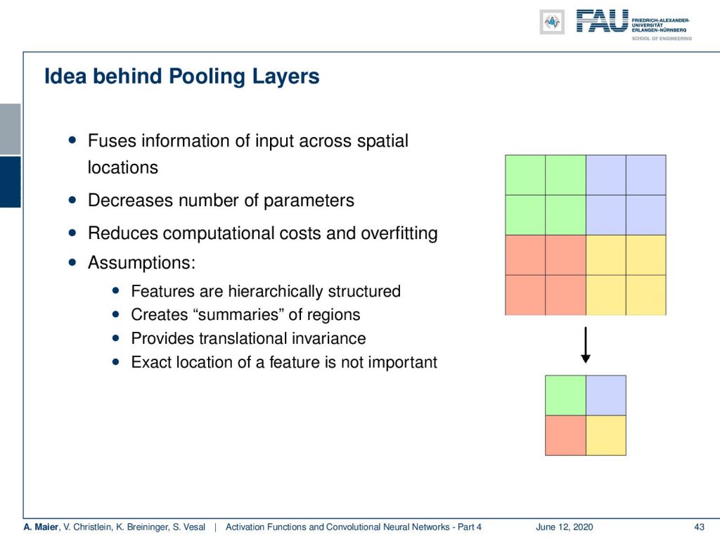
Pooling decreases the spatial information by reduction techniques. Image under CC BY 4.0 from the Deep Learning Lecture.

So here, we see this small example where we summarize the information in the green rectangles, the blue rectangles, the yellow, and the red ones to only one value. So, we have a 2×2 input that has to be mapped onto a single value. Now, this of course reduces the number of parameters. It introduces a hierarchy and allows you to work with spatial abstraction. Furthermore, it reduces computational costs and overfitting. We need some basic assumptions, of course, here and one of the assumptions is that the features are hierarchically structured. By pooling, we’re reducing the output size and introduced this hierarchy that should be intrinsically present in the signal. We talked about the eyes being composed of edges and lines and faces as a composition of eyes and mouth. This has to be present in order to make pooling a sensible operation to be included in your network.

Max pooling selects the maximal index in the receptive field. Image under CC BY 4.0 from the Deep Learning Lecture.

Here, you see a pooling of a 3×3 layer and we choose max pooling. So in max pooling, only the highest number of a receptor field will actually be propagated into the output. Obviously, we can also work with lager strides. Typically the stride equals the neighborhood size such that we get one output per receptive field.

Max pooling only considers the maximum in each receptive field. Fans of ABBA please click here. Image under CC BY 4.0 from the Deep Learning Lecture.

The problem here is of course that the maximum operation adds an additional non-linearity and therefore we also have to think about how to resolve this step in the gradient procedure. Essentially we use again the subgradient concept where we simply propagate into the cell that has produced the maximum output. So, you could say the winner takes it all.

Average pooling is a common alternative to max pooling. Image under CC BY 4.0 from the Deep Learning Lecture.

Now an alternative to this is average pooling. Here, we compute simply the average over the neighborhood. However, it does not consistently perform better than max pooling. In the backpropagation pass, the error is simply shared in equal parts and backpropagated to the respective units.

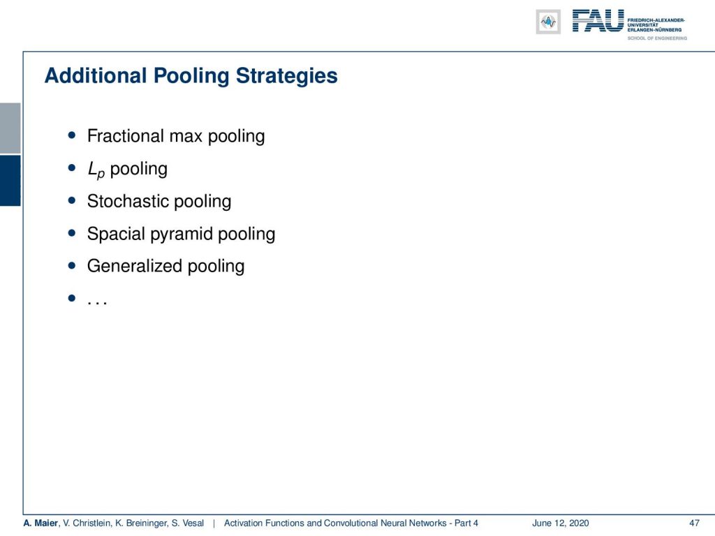
Many other choices for pooling are available. Image under CC BY 4.0 from the Deep Learning Lecture.

There are many more pooling strategies like fractional max pooling, Lp pooling, stochastic pooling, special pyramid pooling, generalized pooling, and many more. There’s a whole different set of strategies about this. Two alternatives that we already talked about are the strided and atrous convolutions. This became really popular because then you don’t have to encode the max pooling as an additional step and you reduce the number of parameters. Typically people now use strided convolutions with S greater than one in order to implement convolution and pooling at the same time.

Typical design choices for a deep network. Image under CC BY 4.0 from the Deep Learning Lecture.

So let’s recap what our convolutional neural networks are doing. We talked about the convolution producing feature maps and the pooling reducing the size of the respective feature maps. Then, again convolutions and pooling until we end up at an abstract representation. Finally, we had these fully connected layers in order to do the classification. Actually, we can kick out this last block because we’ve seen that if we replace this with a reformatting into a channel direction, then we can replace it with a 1×1 convolution. Subsequently, we just apply this to get our final classification. Hence, we can reduce the number of building blocks further. We don’t even need fully connected layers anymore!

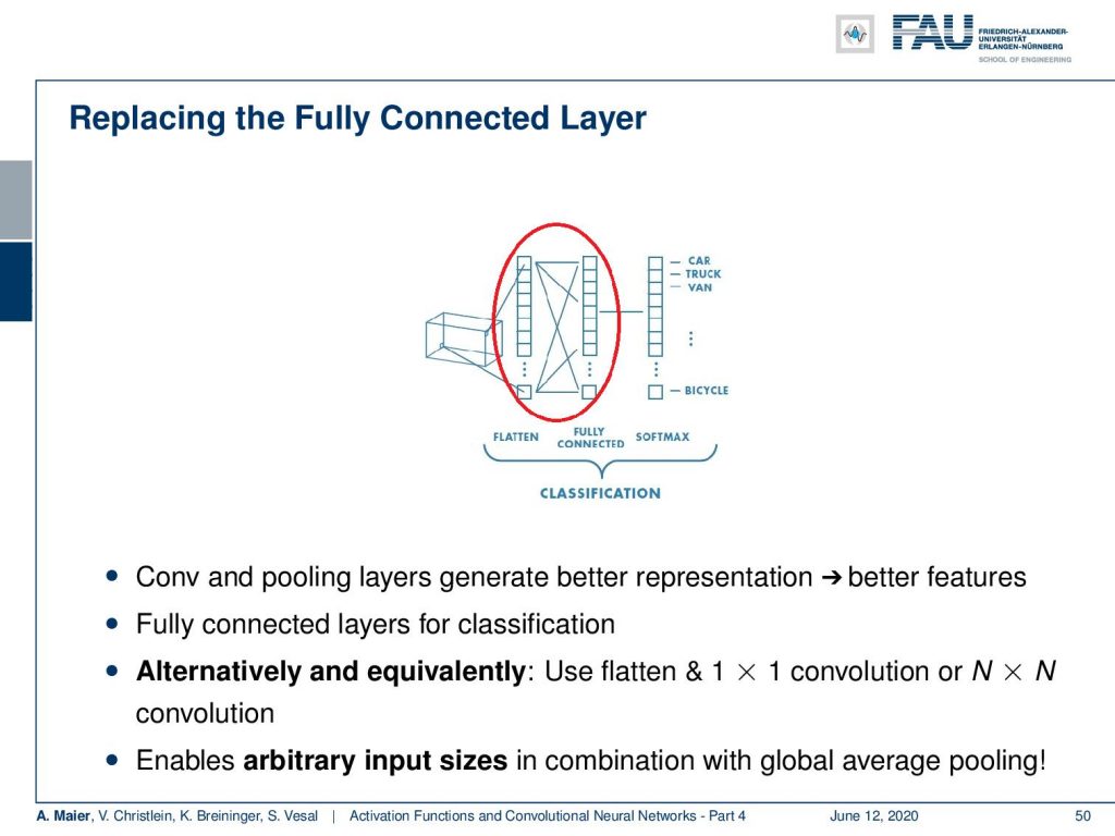
1×1 convolutions are able to replace fully connected layers. Image under CC BY 4.0 from the Deep Learning Lecture.

Now, everything then becomes fully convolutional and we can express essentially the entire chain of operations by convolutions and pooling steps. So, we don’t even need to fully connected layers anymore. The nice thing about using the 1×1 convolutions is if you combine this with something that is called global average pooling, then you can essentially also process input images of arbitrary size. So, the idea here is then that at the end of the convolutional processing you simply map into the channel direction and compute the global average for all of your inputs. This works, because you have a predefined global pooling operation. Then, you can make this applicable to images of arbitrary sizes. So again, we benefit from the ideas of pooling and convolution.

To go even deeper, we will soon look into further ideas. Image under CC BY 4.0 from the Deep Learning Lecture.

An interesting concept that we will also look at in more detail later in this lecture is the inception model. This approach is from the paper “Going deeper with convolutions” [8] following our self-stated motto: “We need to go deeper!”. This network won the ImageNet Challenge 2014. An example is GoogLeNet as one incarnation that was inspired by reference [4].

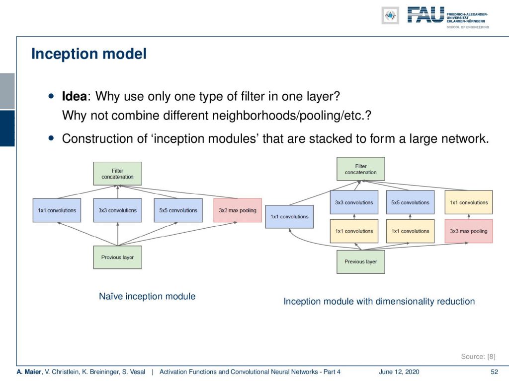
The inception module allows the network to learn the sequence of convolutions and pooling by itself. Image under CC BY 4.0 from the Deep Learning Lecture.

The idea that they presented tackles the problem of having to fix the steps of convolution and pooling in alternation. Why not allow the network to learn on its own when it wants to pool and when it wants to convolve? So, the main idea is that you put in parallel 1×1 convolution, 3×3 convolution, 5×5 convolution, and max pooling. Then, you just concatenate them. Now, the interesting thing is if you offered all four operations in parallel that essentially means that the next layer can then choose what input to trust most in order to construct the deep network. If you do this, then you can further expand this for example at the 3×3 and 5×5 convolutions. You may want to compress the channels first before you actually evaluate them. Then, you find the configuration here on the right-hand side. This incorporates additional dimensionality reduction. Still, this parallel processing allows you to have a network learn on its own sequence of pooling and convolution layers.

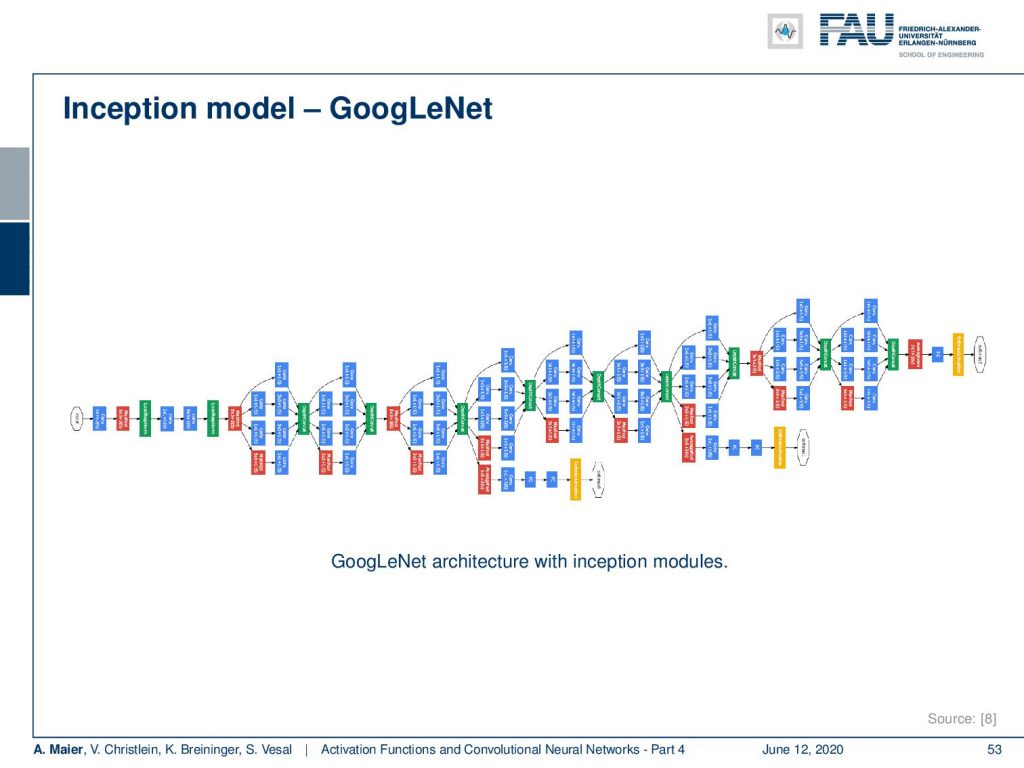
The full GoogLeNet architecture will be described soon in more detail. Image under CC BY 4.0 from the Deep Learning Lecture.

Then, you get models like this one. This is already a pretty deep model that features a lot of interesting further innovations that we will talk about when we are speaking about different network architectures.

More exciting things coming up in this deep learning lecture. Image under CC BY 4.0 from the Deep Learning Lecture.

So next time in deep learning, we want to talk about how we can prevent networks just from memorizing the training data. Is there a way to force features to become independent? How can we make sure our network also recognizes cats in different poses? Also, a very nice recipe that can help you with that and how can we fix the internal covariate shift problem. These are all important points and I think the answers really deserve to be presented here.

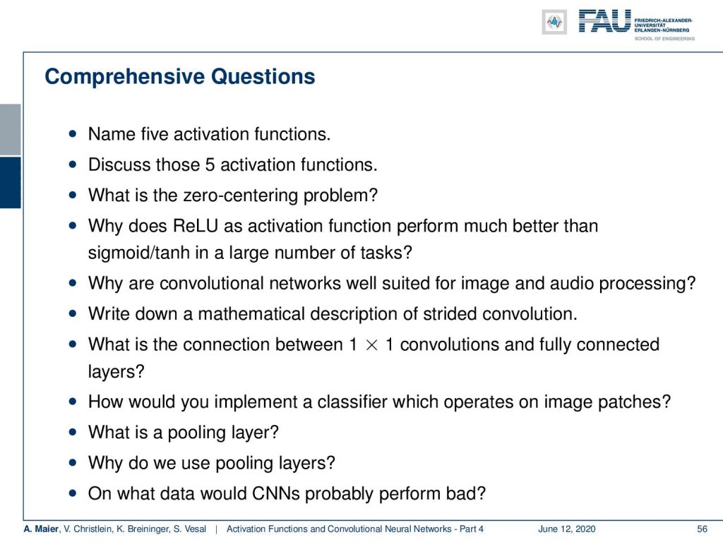
Comprehensive questions may help students to prepare the exam. Image under CC BY 4.0 from the Deep Learning Lecture.

Also, I have a couple of comprehensive questions or tasks. Name five activation functions. Discuss those five activation functions. What is the zero centering problem? Write down a mathematical description of strided convolution. What is the connection between 1×1 convolutions and fully connected layers? What is a pooling layer? Why do we need those pooling layers? So, many interesting things that somebody could ask you at a certain point in time. If you have any questions, you can post them in the comments or send them by email. So, I hope you like this lecture and we’ll see you in the next one!

If you liked this post, you can find more essays here, more educational material on Machine Learning here, or have a look at our Deep Learning Lecture. I would also appreciate a clap or a follow on YouTube, Twitter, Facebook, or LinkedIn in case you want to be informed about more essays, videos, and research in the future. This article is released under the Creative Commons 4.0 Attribution License and can be reprinted and modified if referenced.

References

[1] I. J. Goodfellow, D. Warde-Farley, M. Mirza, et al. “Maxout Networks”. In: ArXiv e-prints (Feb. 2013). arXiv: 1302.4389 [stat.ML].
[2] Kaiming He, Xiangyu Zhang, Shaoqing Ren, et al. “Delving Deep into Rectifiers: Surpassing Human-Level Performance on ImageNet Classification”. In: CoRR abs/1502.01852 (2015). arXiv: 1502.01852.
[3] Günter Klambauer, Thomas Unterthiner, Andreas Mayr, et al. “Self-Normalizing Neural Networks”. In: Advances in Neural Information Processing Systems (NIPS). Vol. abs/1706.02515. 2017. arXiv: 1706.02515.
[4] Min Lin, Qiang Chen, and Shuicheng Yan. “Network In Network”. In: CoRR abs/1312.4400 (2013). arXiv: 1312.4400.
[5] Andrew L. Maas, Awni Y. Hannun, and Andrew Y. Ng. “Rectifier Nonlinearities Improve Neural Network Acoustic Models”. In: Proc. ICML. Vol. 30. 1. 2013.
[6] Prajit Ramachandran, Barret Zoph, and Quoc V. Le. “Searching for Activation Functions”. In: CoRR abs/1710.05941 (2017). arXiv: 1710.05941.
[7] Stefan Elfwing, Eiji Uchibe, and Kenji Doya. “Sigmoid-weighted linear units for neural network function approximation in reinforcement learning”. In: arXiv preprint arXiv:1702.03118 (2017).
[8] Christian Szegedy, Wei Liu, Yangqing Jia, et al. “Going Deeper with Convolutions”. In: CoRR abs/1409.4842 (2014). arXiv: 1409.4842.