Convolutional Layers
These are the lecture notes for FAU’s YouTube Lecture “Deep Learning“. This is a full transcript of the lecture video & matching slides. We hope, you enjoy this as much as the videos. Of course, this transcript was created with deep learning techniques largely automatically and only minor manual modifications were performed. If you spot mistakes, please let us know!
Welcome back to deep learning! Today, we want to continue talking about convolutional neural networks. What we really want to see in this lecture, are the building blocks towards building deep networks. So what we will learn about today are convolutional neural networks, This is one of the most important building blocks of deep networks.
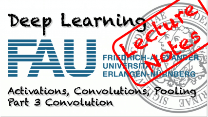
So far, we had those fully connected layers where each input is connected to each node. This is very powerful because it can represent any kind of linear relationship between the inputs. Essentially between every layer, we have one matrix multiplication. This essentially means that from one layer to another layer, we can have an entire change of representation. It also means that we have a lot of connections.
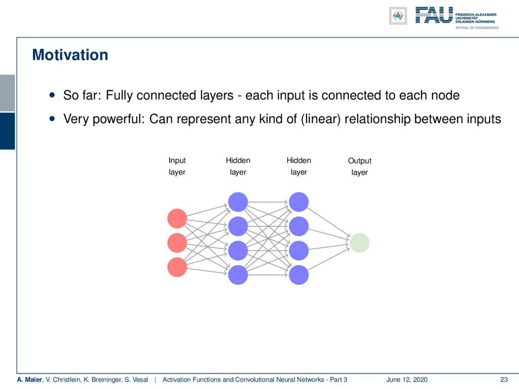
So let’s think about images, videos, sounds, and machine learning. Then, this is a bit of a disadvantage because they typically have huge input sizes. You want to think about how to deal with these large input sizes. Let’s say, we assume we have an image with 512 times 512 pixels that means that one hidden layer with eight neurons has already 512 ^ 2 + 1 for the bias times 8 trainable weights. That’s more than 2 million trainable weights just for a single hidden layer. Of course, this is not the way to go and size is really a problem. There’s more to that.
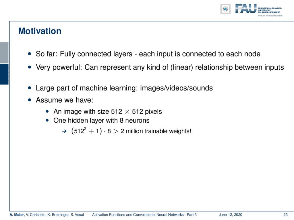
So let’s say we want to classify between a cat and a dog. If you look at those two images, then you can see that a large part of these images, they just contain empty areas. So, they are not very relevant as pixels, in general, are very bad features. They are highly correlated, scale-dependent, and have intensity variations. So they’re a huge problem and pixels are a bad representation from a machine learning point of view. You want to create something that is more abstract and summarizing the information better.
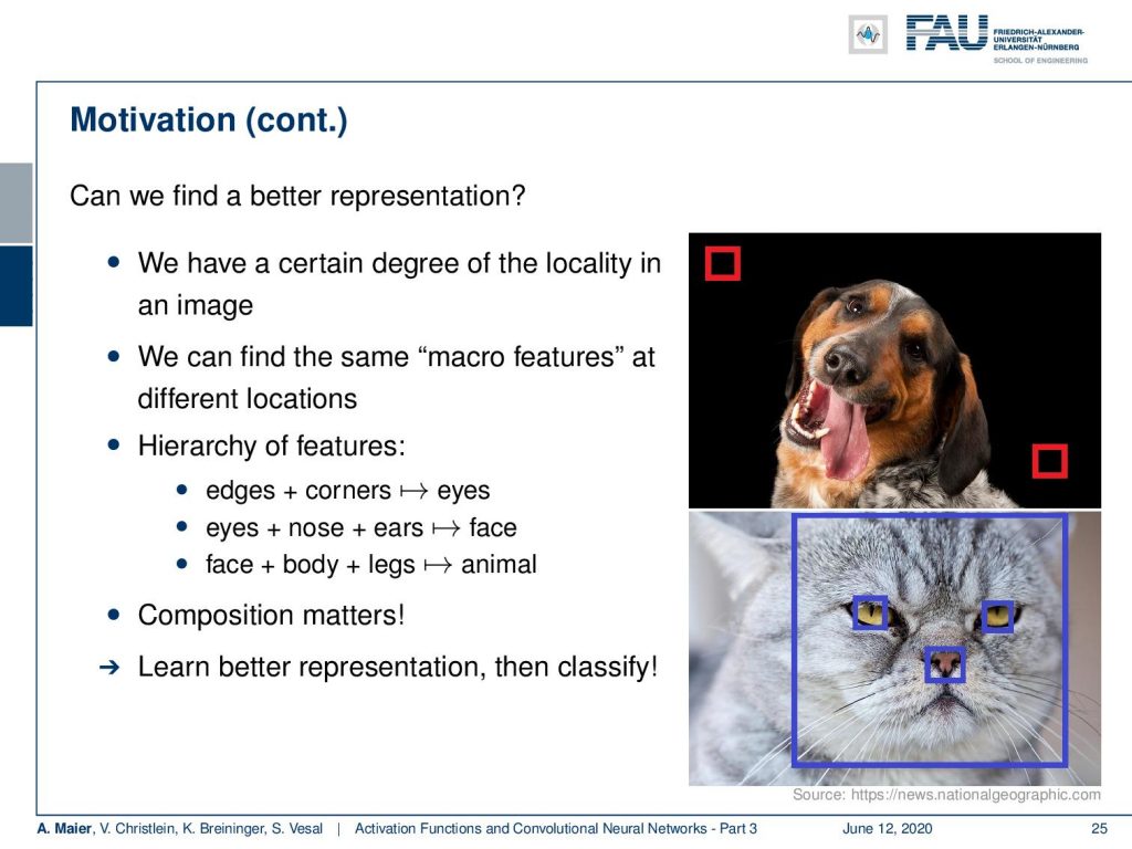
So, the question is: “Can we find a better representation?” We have a certain degree of locality of course in an image. So, we can try to find the same macro features at different locations, and then we reuse them. Ideally, we want to construct something like a hierarchy of features where we have edges and corners that then form eyes. Then, we have, eyes, nose, and ears that form a face, and then face, body, and legs will finally form an animal. So, composition matters and if you can learn a better representation then you can also classify better.
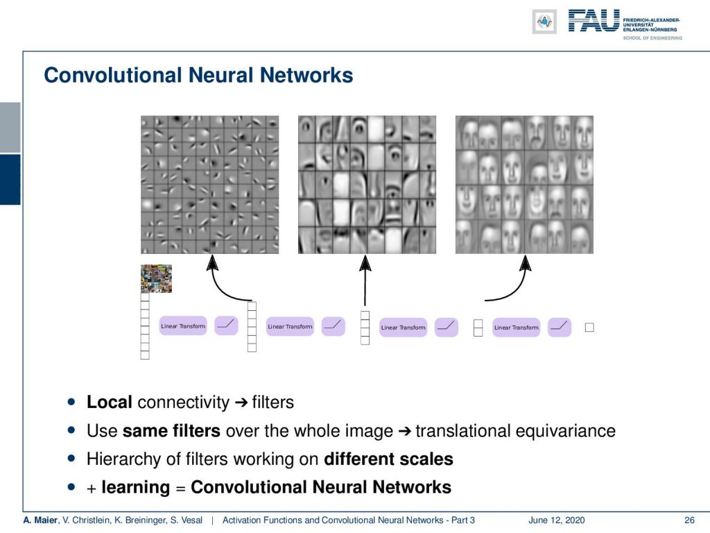
So this is really key and what we often see in the convolutional neural networks is that you find very simple descriptors on the early layers. Then, in the intermediate layers, you’ll find more abstract representations. Here, we find eyes, noses, and so on. In the higher layers, you then find really receptors for example here faces. So, we want to have a local sensitivity but then we want to scale them over the entire network in order to also model these layers of abstraction. We can do that by using convolution in neural networks.
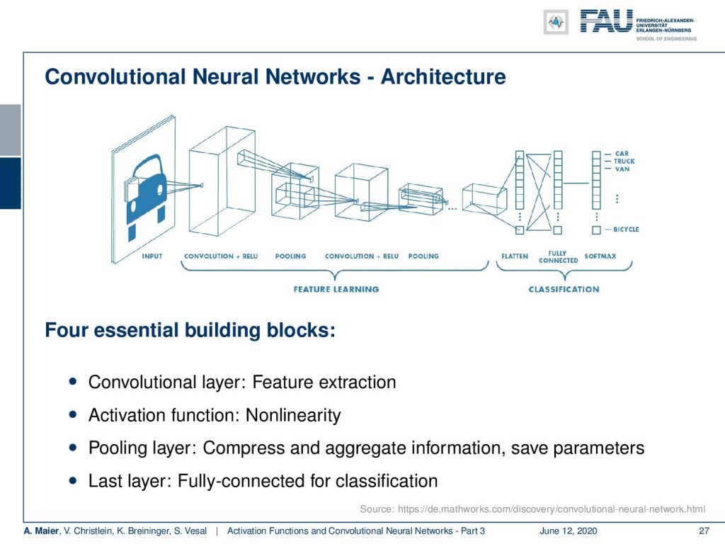
So, here is generally the idea of these architectures. Instead of fully connecting everything with everything, they use a so-called receptive field for every neuron that is like a filter kernel. Then, they compute the same weights over the entire image – essentially a convolution – and produce different so-called feature maps. Next, the feature maps go to a pooling layer. The pooling then tries to bring in the abstraction and de-magnify the image. In the following, we then can again do a convolution and pooling and can go into the next stage. You go on until you have some abstract representation and the abstract representation is then fed to a fully connected layer. This fully connected layer, in the end, maps to the final classes which are “car”, “truck”, “van” and the like. This is then the classification result. So, we need convolutional layers, activation functions, and pooling to get the abstraction and to reduce the dimensionality. In the last layers, we find fully connected ones for classification.
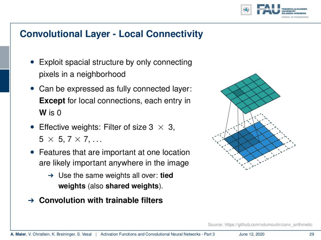
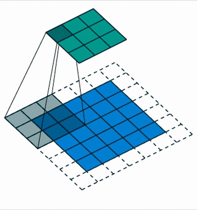
So let’s start with the convolutional layers. So, the idea here is that we want to exploit the spatial structure by only connecting pixels in a neighborhood. This can be then expressed in a fully connected layer except if we want to express this in a fully connected layer, we could set every entry in our matrix to zero except they are connected by local connections. So this would mean that we have can neglect many connections over spacial distances. Another trick is that you use filters of size 3 x 3, 5 x 5, and 7 x 7 and you want them to be identical over the entire layer. So, the weights within the small neighborhood are the same even when you shift them around. They are then called tied or shared weights. If you do this, you are essentially modeling a convolution. If you have the same weights, then this is exactly the same concept that you learn in any image processing class as filter masks, So, we essentially here construct networks that have trainable filter masks.
Here, we see a blow-up view of this process. So, essentially convolution – if you have attended a signal processing class – can be expressed as the integral over two functions where you shift one of the functions over the other and then integrate the final result.
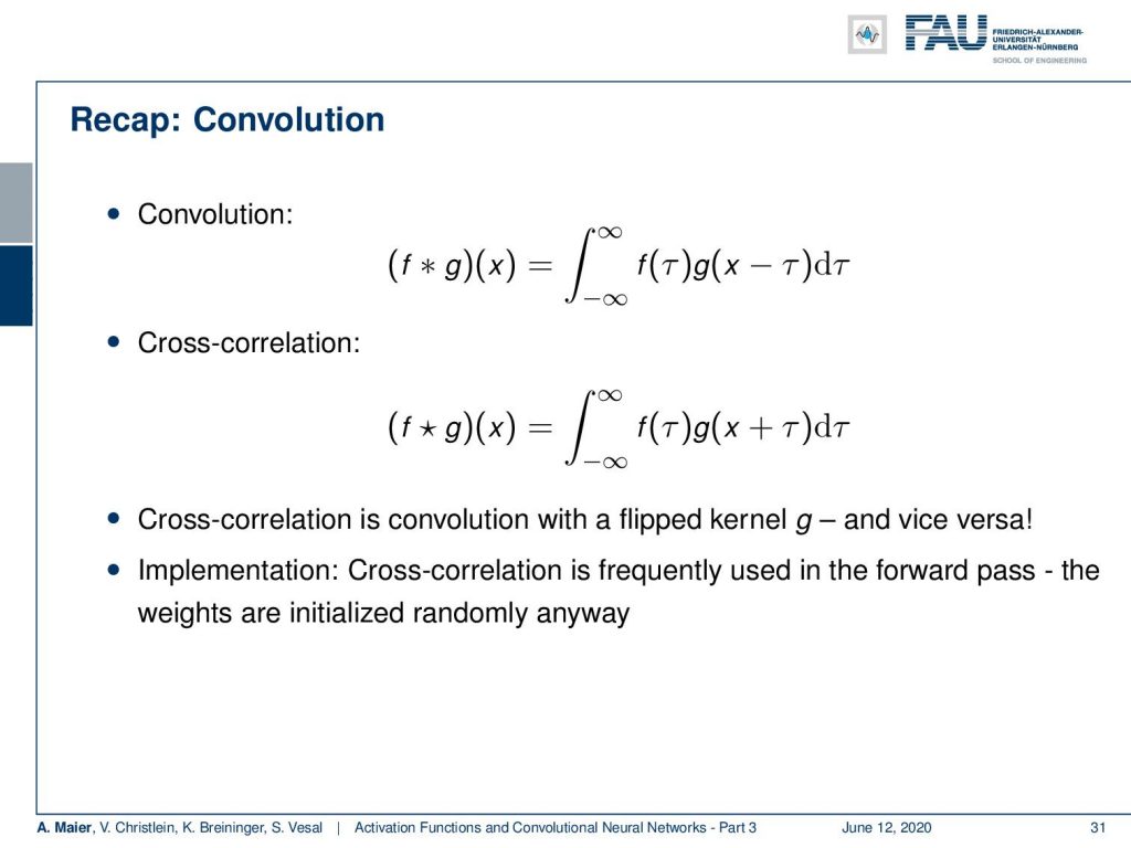
Cross-correlation is an associated concept and you see that the only difference between cross-correlation and convolution is the sign for τ. In convolution, you move in a negative direction, and in cross-correlation, you move in a positive direction. What we see quite often is that people talk about convolutions, but they actually implemented cross-correlation. So they essentially flipped the direction of the mask. So, if you are creating something that is trainable, it actually doesn’t matter because you would learn the sign of the function anyway. So, both implementations will be fine. Cross-correlation is actually frequently being implemented in actual deep learning software. Typically, you initialize the weights randomly anyway. Hence, the difference has no effect.
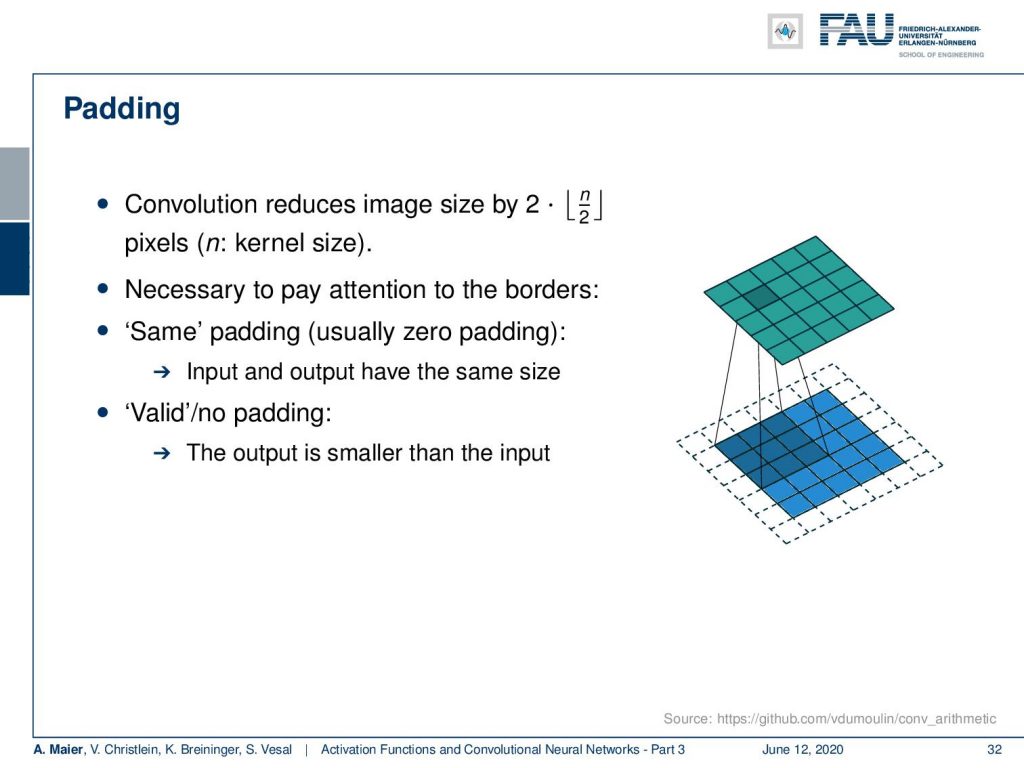
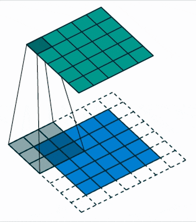
Another thing that we need to talk about is different input sizes and how the convolution is actually then being used to process. So this receptive field implies that the output is actually smaller because we have only access to the very up to the very boundary. So, if you want to compute the convolution kernel at the very boundaries of your receptive field, you would actually reach outside of the field of view. One way of dealing with this is then to reduce the size of the feature map and the next respective layer. You can also use padding. What many people do is just zero padding. So, all values that have not been observed are actually set to zero and then you can remain in the same size and just convolve the entire image. There are also other strategies like mirroring and so on but zero padding is probably the most common one.
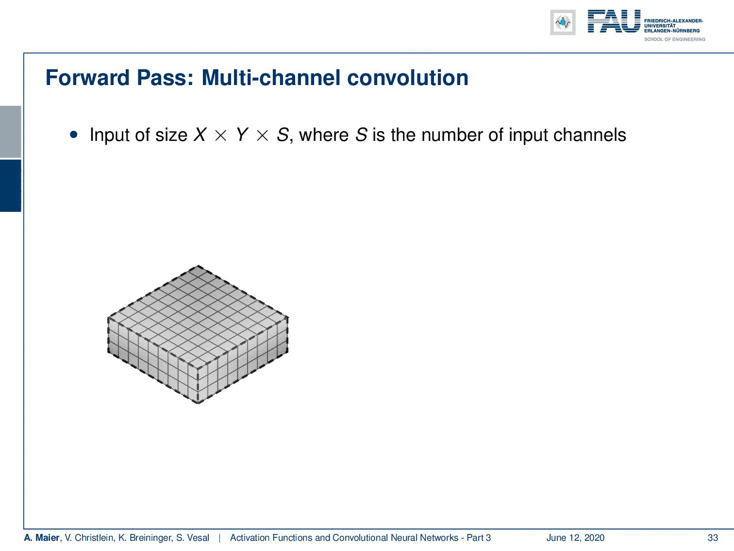
This way, you get the forward path. You actually don’t have to implement it with the small convolution kernels. You can also use a Fourier transform to actually perform the convolution. So, you have a 2-D input image. Let’s say it’s a multi-channel image where for example S is the number of colors. Then, you apply a 3-D filter. Here, you can see that in the spatial domain you have the convolution kernel but in S direction it’s fully connected across the channels. If you do so, you can apply this kernel and then you get exactly one output mask (shown in blue) with the kernel shown here. Then, we return here this single output field. Now, if you had another kernel, then you can produce a second mask with the same padding as shown in green. This way, you can then start constructing one feature map after another.
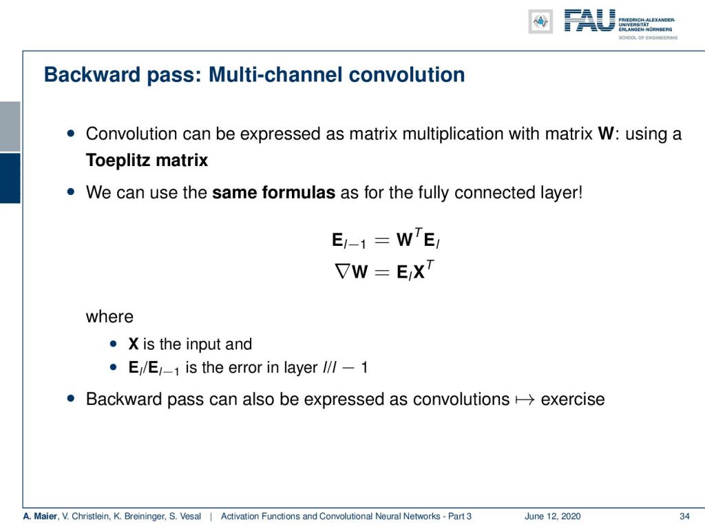
Let’s talk a bit about convolution implementation and the backward pass. Convolution is expressed as a matrix multiplication W and W is a Toeplitz matrix. So, this Toeplitz matrix is a circulant matrix as it is constructed by weight sharing. This means that if you are actually constructing this matrix, you have essentially the same number of weights in every row that is being trained, but they are shifted by one just because they are computing a different local field in every row using the same weights. So this gives us a circulant matrix and it means that we stay in the domain of matrix multiplication. So also our convolution can be implemented as matrix multiplication and therefore we simply inherit the same formulas as for the fully connected layer. So if we want to backpropagate the error, it’s simply W transposed times the input error from the backpropagation. If you want to compute the update for the weights, it’s essentially the error term multiplied with what we got from the input in the forward pass transposed. So, it’s exactly the same update formulas as we have seen them previously for fully connected layers. This is nice and there’s not so much to keep in mind. Of course, you have to make sure that you get this weight sharing implemented correctly which we’ll show you in the exercises. For us now, we can just treat it as matrix multiplication and one interesting thing that you see in the exercises is by the way that the backward pass can also be expressed as convolution.
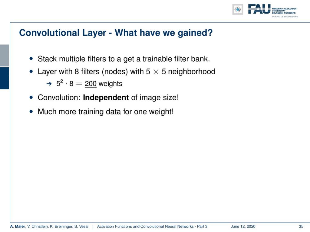
Now, what have we gained with the convolutional layers? Well, if now stack multiple filters, we get essentially a trainable filter bank. Let’s say, we have eight filters resulting in eight nodes and a 5×5 neighborhood. Then, we suddenly have 5^2 times 8 = 200 weights. 200 weights are considerably less than the two million weights that we’ve seen before. Also, convolution can be applied independently of the image size. So, what we can do is we can convert any kind of image with those filters. It means that the activation maps that we are producing also change when we have a different input size. We will see more of that in one of the next lectures. The very nice thing here is that we have much more data to train a single weight.
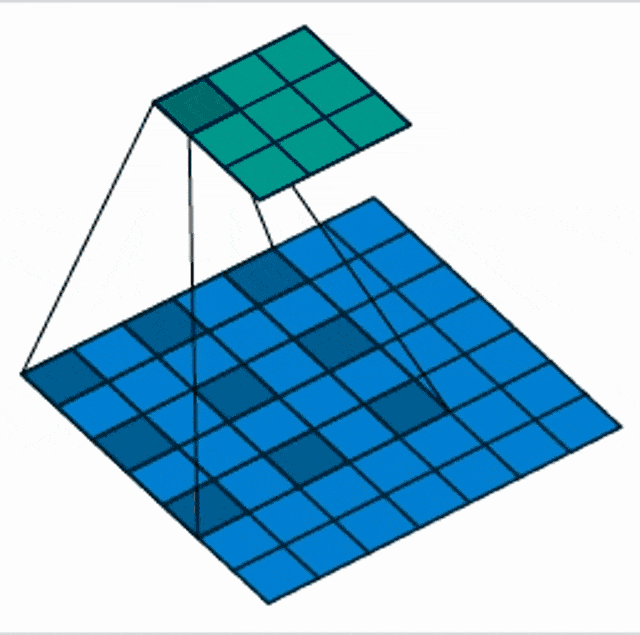
There are also things like the strided convolutions. This is when you try to incorporate the pooling mechanism and the dimensionality reduction mechanism into the convolution. It’s like skipping one step at each point. So, with the stride s, we describe an offset and then we intrinsically produce an activation map that has a lower dimension that is dependent on this stride.
So, we reduce the size of the output by a factor of s because skipping so many steps and mathematically this is simply convolution and subsampling at the same time. We have this small animation here in order to show you how this is being implemented.
There are also things like dilated our atrous convolutions. Here the idea is that we are not increasing the stride but we are increasing the spacing the input space. Now, the receptive field is no longer connected but we are looking at individual pixels spread over a neighborhood. This then gives us a wider receptive field with fewer parameters.
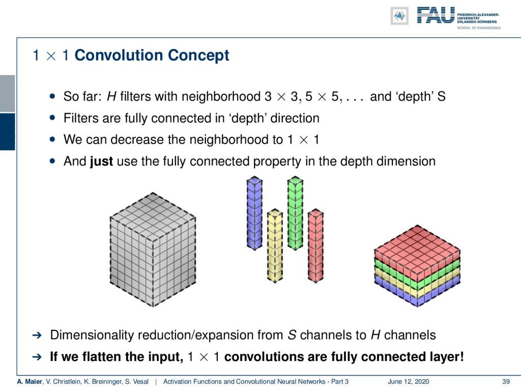
Another very interesting concept is the 1×1 convolution. So far, we had H filters with these neighborhoods and in depth direction, we had S. Remember, they were fully connected in the depth direction. This is also interesting because now if you have a 1×1 convolution, then this is essentially the same as a fully connected layer. So you simply have a fully connected layer over the single dimension and you can then put an arbitrary input. What it does is it computes a reduced number of feature maps in the direction of the channels because there we have the full connection. So essentially, we can now do a channel compression. With 1×1 convolutions, we can flatten the input to one dimension and map everything into the channel direction. Thus, 1×1 convolutions are fully connected layers. So, we can essentially express also the entire concept of fully connected layers with them if we arrange the outputs in an appropriate way.
So this was first described in the network in network paper [4] that we will also talk about when we talk about different architectures. These 1×1 convolutions, decrease the size of a network in particular to compress the channels and it intrinsically learns the dimensionality reduction. Thus, they help you to reduce redundancy in your feature space. Equivalent, but more flexible are of course NxN convolutions.
So next time in deep learning, we will talk about the pooling mechanism and how to reduce the size of the feature maps instead of using convolutions strided or atrous convolutions. You can also model this explicitly in the pooling step which we will talk about in the next lecture. So thank you very much for listening and see you in the next lecture!
If you liked this post, you can find more essays here, more educational material on Machine Learning here, or have a look at our Deep Learning Lecture. I would also appreciate a clap or a follow on YouTube, Twitter, Facebook, or LinkedIn in case you want to be informed about more essays, videos, and research in the future. This article is released under the Creative Commons 4.0 Attribution License and can be reprinted and modified if referenced.
References
[1] I. J. Goodfellow, D. Warde-Farley, M. Mirza, et al. “Maxout Networks”. In: ArXiv e-prints (Feb. 2013). arXiv: 1302.4389 [stat.ML].
[2] Kaiming He, Xiangyu Zhang, Shaoqing Ren, et al. “Delving Deep into Rectifiers: Surpassing Human-Level Performance on ImageNet Classification”. In: CoRR abs/1502.01852 (2015). arXiv: 1502.01852.
[3] Günter Klambauer, Thomas Unterthiner, Andreas Mayr, et al. “Self-Normalizing Neural Networks”. In: Advances in Neural Information Processing Systems (NIPS). Vol. abs/1706.02515. 2017. arXiv: 1706.02515.
[4] Min Lin, Qiang Chen, and Shuicheng Yan. “Network In Network”. In: CoRR abs/1312.4400 (2013). arXiv: 1312.4400.
[5] Andrew L. Maas, Awni Y. Hannun, and Andrew Y. Ng. “Rectifier Nonlinearities Improve Neural Network Acoustic Models”. In: Proc. ICML. Vol. 30. 1. 2013.
[6] Prajit Ramachandran, Barret Zoph, and Quoc V. Le. “Searching for Activation Functions”. In: CoRR abs/1710.05941 (2017). arXiv: 1710.05941.
[7] Stefan Elfwing, Eiji Uchibe, and Kenji Doya. “Sigmoid-weighted linear units for neural network function approximation in reinforcement learning”. In: arXiv preprint arXiv:1702.03118 (2017).
[8] Christian Szegedy, Wei Liu, Yangqing Jia, et al. “Going Deeper with Convolutions”. In: CoRR abs/1409.4842 (2014). arXiv: 1409.4842.