Lecture Notes in Pattern Recognition: Episode 27 – Kernel PCA and Sequence Kernels

These are the lecture notes for FAU’s YouTube Lecture “Pattern Recognition“. This is a full transcript of the lecture video & matching slides. We hope, you enjoy this as much as the videos. Of course, this transcript was created with deep learning techniques largely automatically and only minor manual modifications were performed. Try it yourself! If you spot mistakes, please let us know!

Welcome back to pattern recognition. Today we want to look into a couple of the advanced kernel tricks and in particular, we want to introduce the kernel PCA and we want to look into some kernels that can also work on sequences. So looking forward to showing you some advanced methods of pattern recognition.

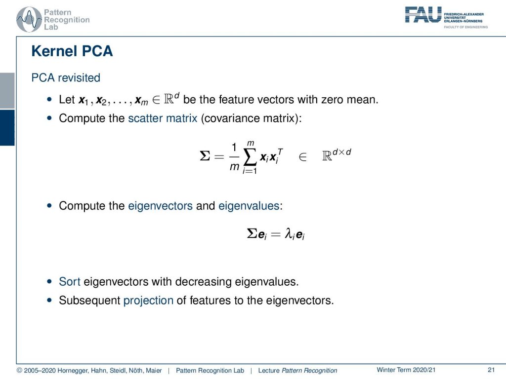
So let’s revisit the PCA. We had some observations x₁ to x_m in a d-dimensional feature space and they have a zero mean. If they don’t have a zero mean then we could of course enforce them to have zero mean by normalization. If we do so we can then compute the scatter matrix or the covariance matrix that is then given as essentially the outer products of the respective feature vectors. This is then a d times d matrix. So this has squared the dimension of the input domain of the features. So we could compute the eigenvectors and eigenvalues of this and this is essentially determined from this eigenvector problem here. Then we sort the eigenvectors with decreasing eigenvalues and this then allows us to use them to project the features into the eigenvalues. 

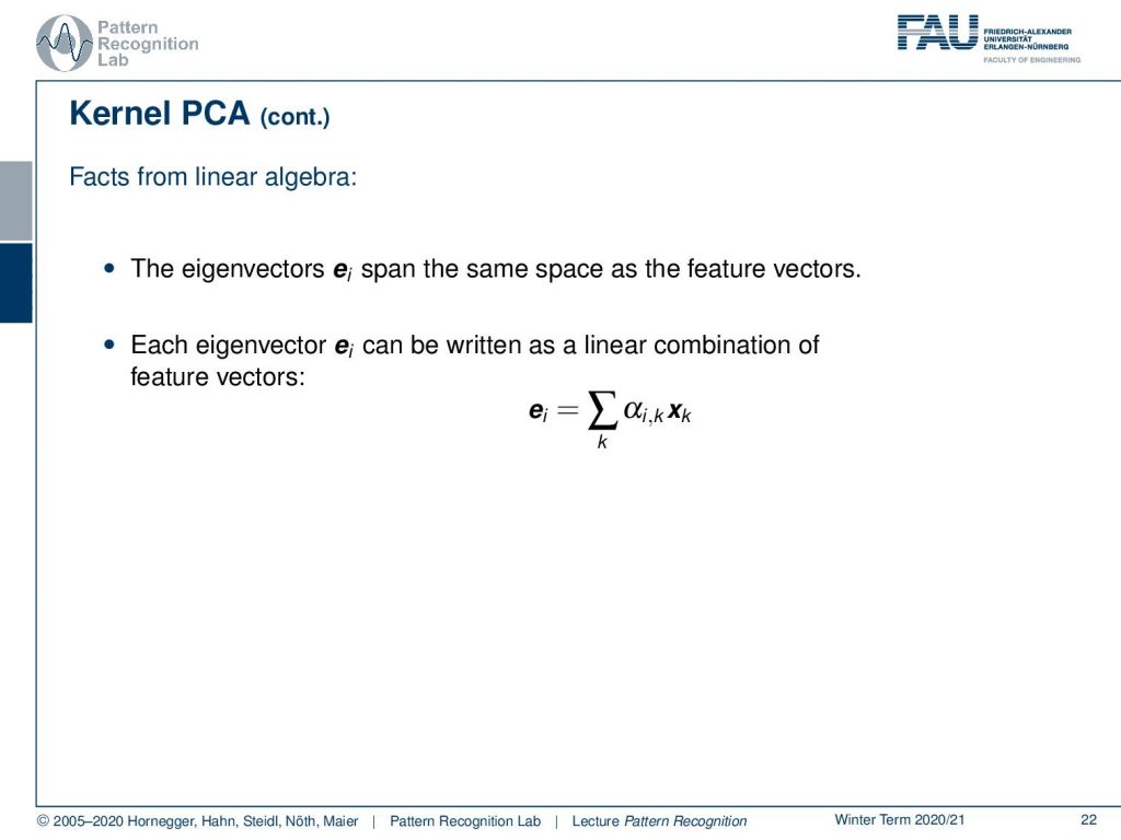
So let’s look into some facts from linear algebra. The eigenvectors expand the same space as the feature vectors. The eigenvectors can be written as a linear combination of feature vectors. So our e_i can be expressed as a linear combination given some α and the respective observations x. 

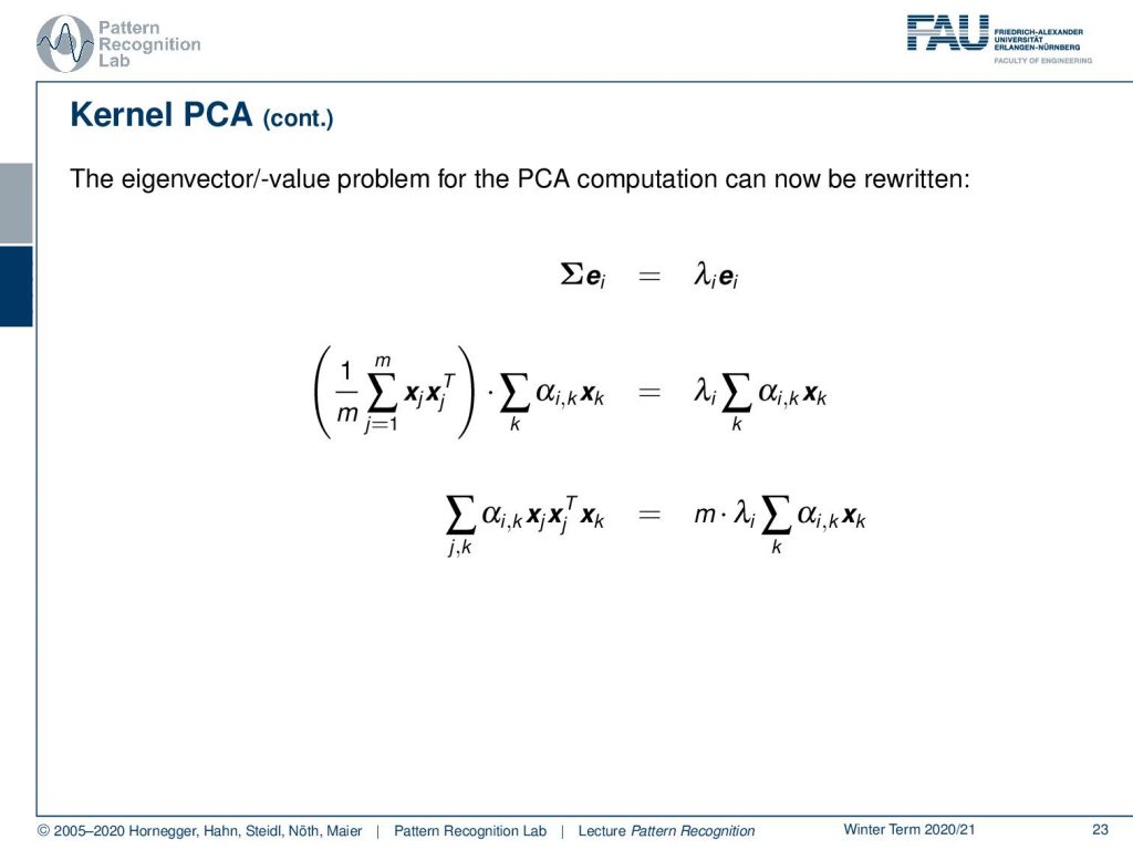
So this means that we can now rewrite the eigenvector eigenvalue problem for the PCA in the following way: So we replace the eigenvectors with the previous definition. This is on the one hand side we see that we replace the scatter matrix with this outer product and we see that we replace the eigenvectors with this αx sum and we also do that on the right-hand side. If we do so we can rearrange this a little bit we can bring the sums on the left-hand side together. We can also bring the m on the other side of the equation. 

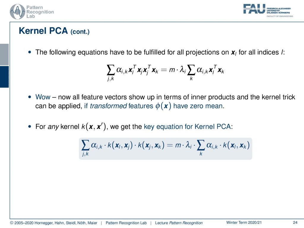
Now let’s look at this in a little more detail and in particular if we have some additional feature vector l now. We multiply transpose from the left-hand side we get the following equation. If you look at this then everything now in terms of feature vector turns out to be inner products. So we have the inner product and the kernel trick can be applied if the transform features have a zero mean. Now for any kernel, we then get the key equation for the kernel PCA that is it’s the sum over the product of the kernels. This is equal to the sum of the αs times the kernel again. So this is the key equation. 

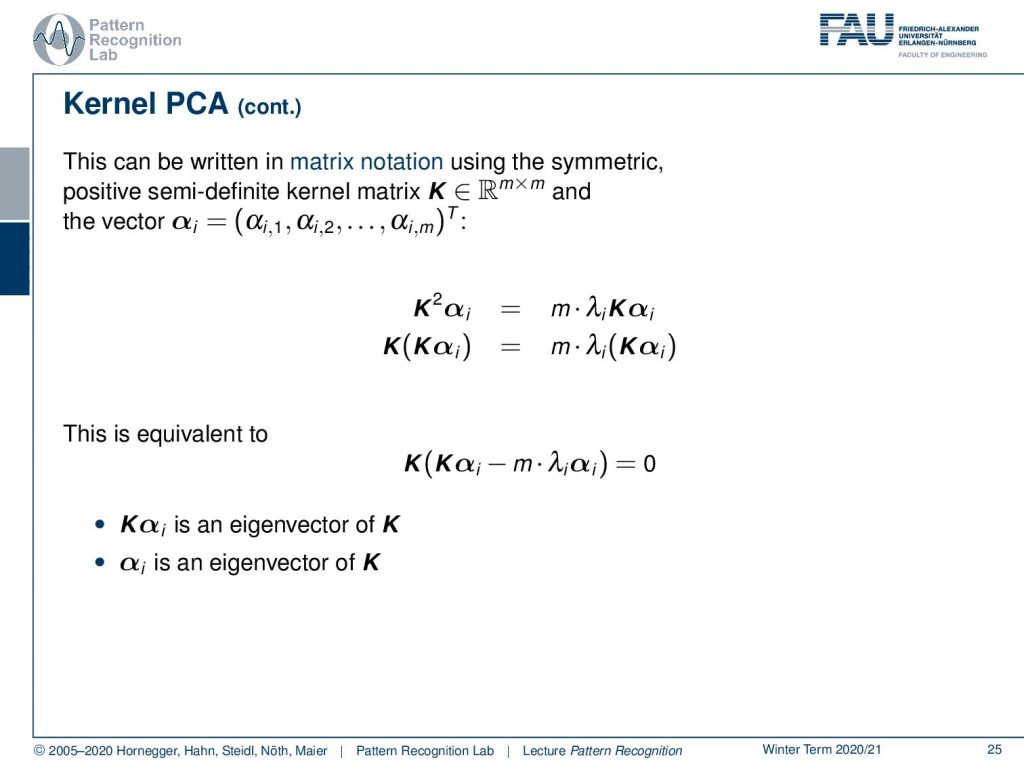
We can now see that in this equation essentially the kernel matrix pops up. So let’s rearrange this a bit into matrix notation then we get rid of the sums and we introduce again our symmetric positive semi-definite kernel matrix K. It is now only in an m times m space. So m times m is essentially the domain of the number of feature vectors. So we essentially are here limited by the number of observations and no longer by the dimensionality of the original feature vectors. Now we see here that we can pull out K on both sides and this is equivalent to bringing everything on one side. You can also pull out K and there you see then that Kα is an eigenvector of K and also that α is an eigenvector of K. So this is essentially an eigenvector problem that we’re writing up here. 

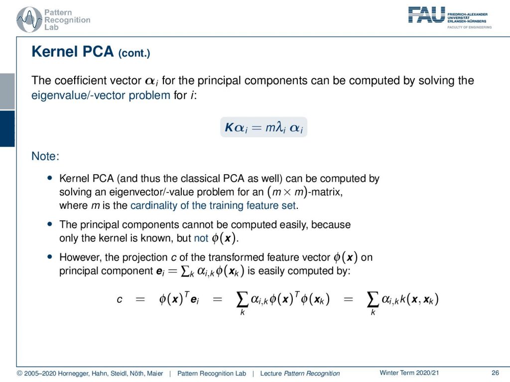
Also, if you would apply the inverse of K to the first line on this slide then you would see that we also come up with this eigenvalue eigenvector problem of the kernel matrix K. Then our αi’s are essentially the eigenvectors. So we can see that we can now solve this and find our principal components. Now observe here that the kernel PCA and by the way also the classical PCA can be computed by solving these eigenvector eigenvalue problems for m times m matrices. Now m is only the cardinality of the training feature set and no longer the dimensionality of the input space. So this is actually a pretty cool property. Then also observe that the principal components cannot be computed that easily because only the kernel is known but not the ϕ(x). So this is generally a property of the kernel PCA here, but we can compute the projection c of the transformed feature vector on the principal component. If we express this now with the feature transform we can see that we can essentially get the c as the eigenvector times the transformed feature. Then we can see that we can express again the eigenvector as the sum of the transformed vectors. There you then see that we have an inner product of the feature transforms again and this brings us back to our kernel function. So we can essentially compute the projection onto the transformed feature vector using the kernel function again. Of course, we need to know our αs’ that we determined from the eigenvector problem above. So this is pretty neat. So we can compute those projections quite easily and this is done using the kernel matrix. 

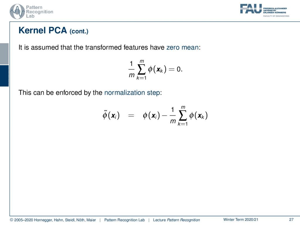
Now if we assume that we have a zero mean then we can also see that we can generate transformed feature vectors by essentially subtracting the mean of the feature vectors from the feature vector after the transformation. This will give us then some ϕ tilde of x_i that is producing essentially feature vectors that are zero centered. Now again here we need the feature transform in order to perform this. 

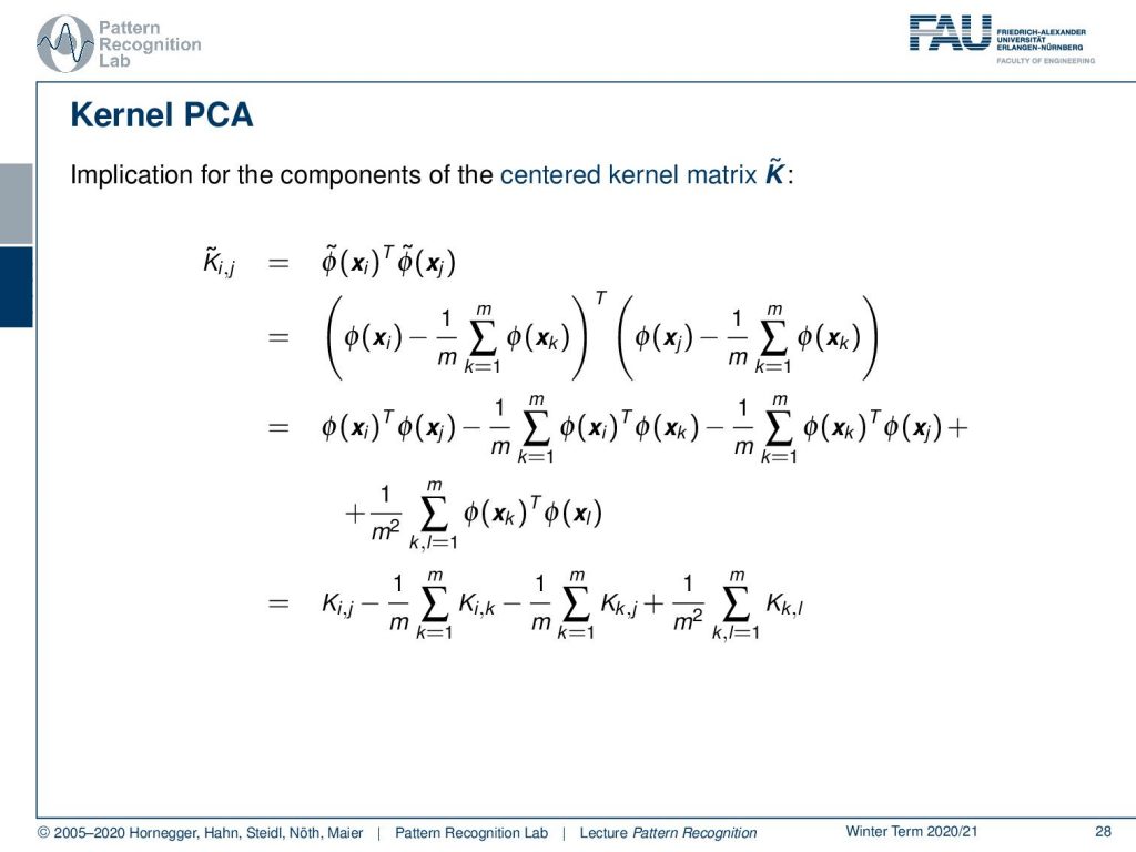
Let’s look into this in a little bit more detail and see what implications we have here for the centered kernel matrix. So we can write this up again as the inner product of our feature transforms of the transformed space. Then we can plug in the definition of ϕ tilde where we have to subtract the means. We see this is essentially an inner product of two long vectors and we can now do the math and take them out. Here you can see that we essentially end up with inner products over the feature transformed vectors. So technically if we want to compute this term we can also rewrite this with respect to the kernel function. So we can compute all of these terms only using the kernel function and therefore we can also produce a centered matrix using only the kernel function. So this is also a very important property because otherwise, we might run into problems with our kernel PCA because we assumed it to be centered.

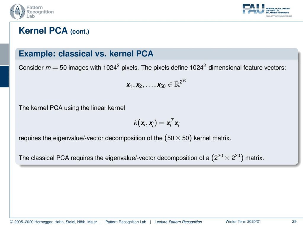
Now let’s look into some examples. let’s consider an image and we have like 50 training observations and we have 1024 to the power of two pixels. Then this means that the input feature vectors define essentially 50 observations in a space that is R to the power of 2 to the power of 20. So this is a very high dimensional space. Now if we use the kernel PCA instead we see that our kernel matrix essentially lives in a 50 times 50 space and this is really something where we still can compute an eigenvalue decomposition. So this is really possible to work with that and now the classical version would actually have to solve the eigenvalue decomposition of a 2 to the power of 20 times 2 to the power of 20 matrix, which is super huge but if we work with the kernel trick here it’s only a matrix that is 50 times 50. So this is a much smaller problem to work with. So here also the kernel PCA has a lot of advantages.

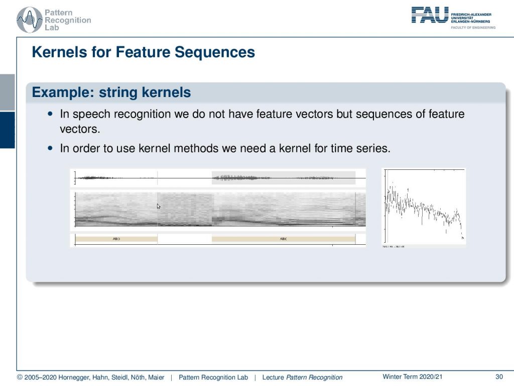
Now we can also apply kernels to strings and for example, in speech, we very often have the problem that we have sequences of different lengths. So if you have time series then you really have a problem. If you have speech signals then you don’t have the same dimensionality for the different feature observations. 

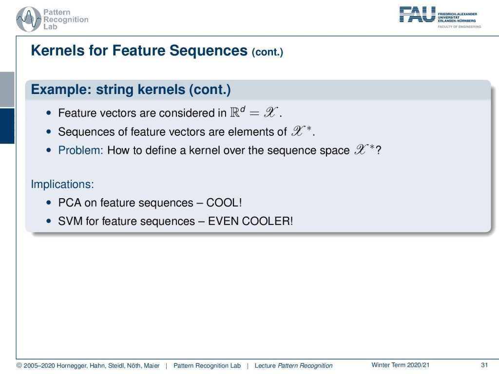
We can still use kernels and there we can then even compare sequences of symbols like strings like waveforms and all kinds of time series data with a kernel space. So we can then even compute PCA on feature sequences which is pretty cool. We can also use SVMs on feature sequences which is even cooler. So everything that we learned on a fixed dimensional feature space right now we can also apply to sequences of varying length. 

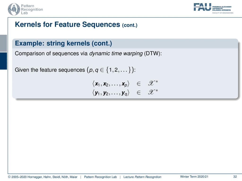
So that is really nice and the key concept here that we will use is the comparison of the sequences using dynamic time warping. So here we have two feature sequences that essentially have a length of p and q. They live in the same feature space but they have different lengths of observations and this is then able to describe a distance using dynamic time warping and here we essentially take the sum over the euclidean distances between the matching observations. 

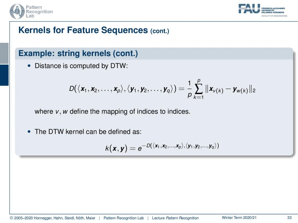
So we use dynamic time warping to compute indices that are matched together. Then those are subtracted from each other and you take the two norm. This gives you a distance. Now with this, we have a distance for different feature sequences and this distance can then be mapped into a kernel function by taking e to the power of minus d as the actual kernel function. So using this trick we can now suddenly define any kind of sequence of feature vectors for symbols for all these kinds of problems. We can define kernel PCA and SVMs. Pretty cool isn’t it.

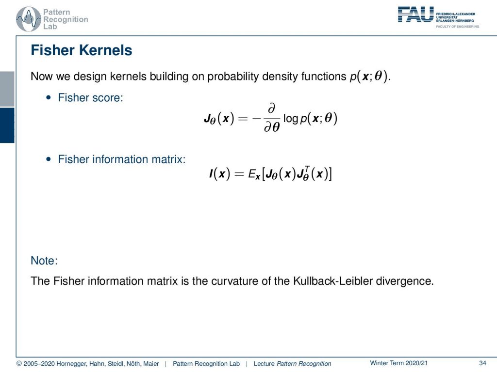
Well what else we can also look into the so-called Fischer kernel. So there we can even construct kernels for probability density functions and this is using the so-called Fisher score where you compute the negative partial derivative with respect to theta of the logarithm of the probability density function. This can then be employed to compute for example the Fisher information matrix I of x that is the expected value of the Fisher scores times the Fisher scores transposed. This is then essentially describing the curvature of the Kullback-Leibler divergence. So both of these concepts can then be used to define kernels. 

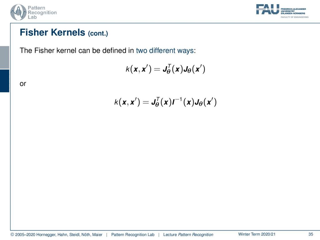
Now the Fisher kernels then can be written in two ways: so you either take the inner product of the Fisher scores or you take the inner product and you weight it with the Fisher information matrix. So these are the two variants that you can get for Fisher kernels. 

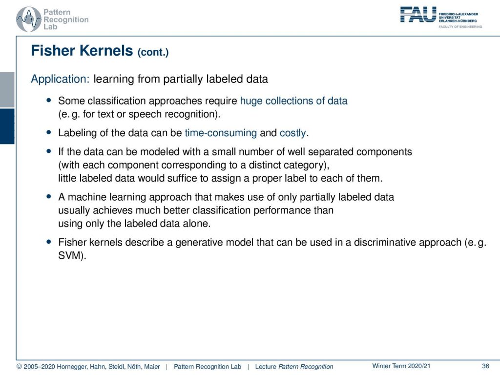
So we can also apply this for example to learning from partially labeled data. So in some classification approaches, you require huge collections of data. So let’s say the text of speech recognition then you label the data and this is super time consuming and costly. If you want to label or transcribe one hour of speech that takes 10 hours of manual labor to actually create the transcription. So if the data can be modeled with a small number of well-separated components with each component corresponding to a distinct category. Then little label data would suffice to assign a proper label to each of them. So a machine learning approach that makes use of only partially labeled data usually achieves much better classification performance than using only the label data alone. The Fisher kernels then describe a generative model that can be used in a discriminative approach for example the support vector machine. 

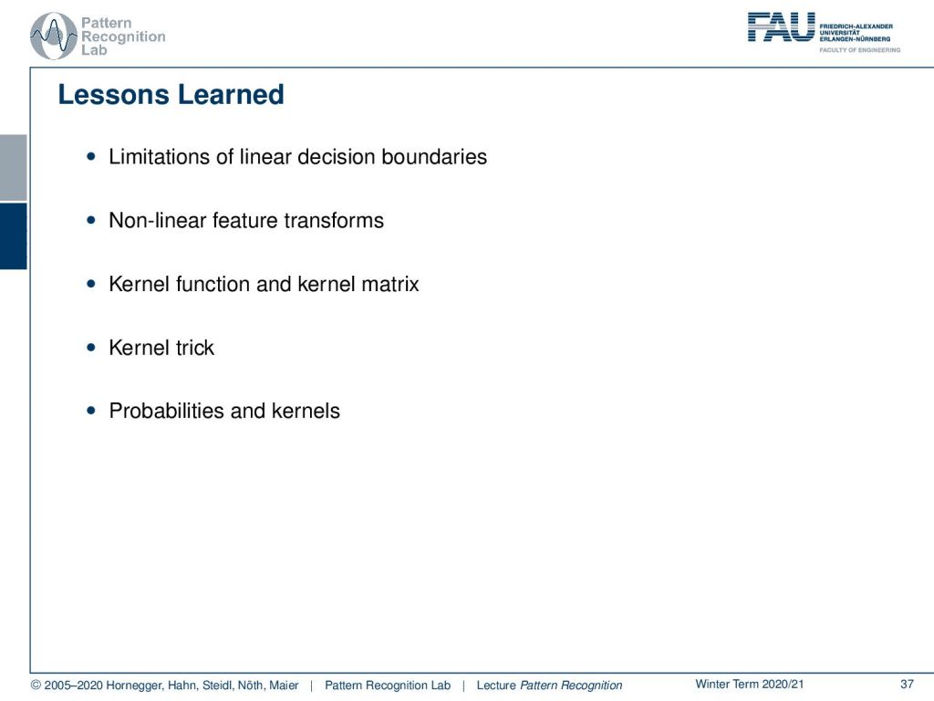
So some lessons learned here about kernels. We have of course strong limitations of linear decision boundaries we’ve seen that there are non-linear feature transforms ranging from polynomials, radial basis functions to even sophisticated ones like string kernels and dynamic time warping. All of them can be applied in the kernel trick and we’ve seen that support vector machines, as well as pca, can embed this kernel trick, and then you can also derive very new transforms that make use of that specific kernel that you have been considering. So this is a really interesting approach and of course, you can also use kernels for probability density functions.

Okay so next time in pattern recognition we want to talk a bit more about an advanced support vector machine and we’ll talk about the laplacian support vector machine. 

So I also have some further readings that are the book by Schölkopf and Smola Learning with Kernels, Vapnik’s The Nature of Statistical Learning Theory and also a very good book is Kernel Methods for Pattern Analysis. 

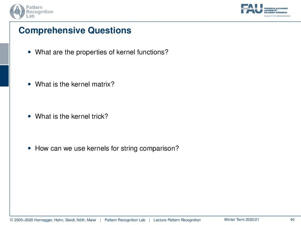
Again, I have some comprehensive questions for you that you will find useful for the exam preparation. This already brings us to the end of this small video. I hope you liked it and I hope you learned something useful in particular that we can also apply kernels to strings and time series and I’m looking forward to seeing you in the next video thank you very much and bye-bye!!!

If you liked this post, you can find more essays here, more educational material on Machine Learning here, or have a look at our Deep Learning Lecture. I would also appreciate a follow on YouTube, Twitter, Facebook, or LinkedIn in case you want to be informed about more essays, videos, and research in the future. This article is released under the Creative Commons 4.0 Attribution License and can be reprinted and modified if referenced. If you are interested in generating transcripts from video lectures try AutoBlog

References

1. Bernhard Schölkopf, Alexander J. Smola: Learning with Kernels, The MIT Press, Cambridge, 2003. 
2. Vladimir N. Vapnik: The Nature of Statistical Learning Theory, Information Science and Statistics, Springer, Heidelberg, 2000.
3. John Shawe-Taylor, Nello Cristianini: ☞ Kernel Methods for Pattern Analysis, Cambridge University Press, Cambridge, 2004

Kategorie: Lecture Notes in Pattern Recognition