
These are the lecture notes for FAU’s YouTube Lecture “Pattern Recognition“. This is a full transcript of the lecture video & matching slides. We hope, you enjoy this as much as the videos. Of course, this transcript was created with deep learning techniques largely automatically and only minor manual modifications were performed. Try it yourself! If you spot mistakes, please let us know!
Welcome back to pattern recognition. Today we want to look a bit more into optimization and the topic today will be looking into the actual update direction. We’ve seen the gradient descent methods in the previous video and today we want to have a couple of thoughts on how to pick the particular update direction.
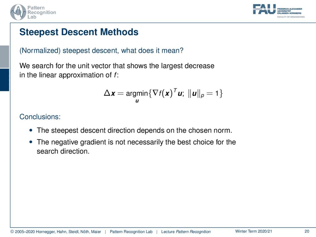
These are different kinds of steepest descent methods and even the normalized ones we might want to consider what update direction we actually want to choose. What we actually want to get is the largest decrease in the linear approximation of f. Technically we could also constrain this gradient direction by a unit ball of an Lp norm. So here we would then search for the update direction as the minimum over sum u that has a length of one according to our norm. Then the projection of the gradient onto this norm. So we observe that if we do this kind of optimization for selecting the update direction, then the steepest direction might not be simply the negative gradient direction. But it may depend on the chosen norm. So the negative gradient is not necessarily the best choice for the search direction.
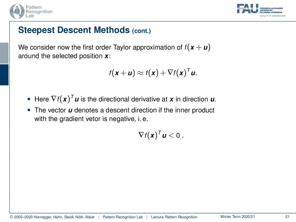
Let’s look into a bit of an idea of how to perform this and here we want to think about some linear ideas. We consider now the first-order Taylor approximation of f(x+u). If we want to look at that in the selected position x then we can approximate f(x+u) as f(x) plus the gradient of f(x) inner product with this unit ball u. So here this inner product of the gradient and the unit ball is the directional derivative of x in direction u. So the vector u denotes a descent direction. If the inner product with the gradient vector is negative which means that we have this inner product smaller than zero.
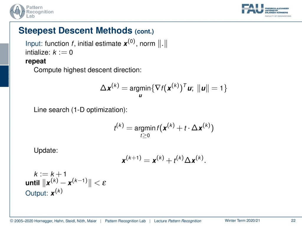
Now this gives then rise to a new steepest descent method. We again have the function we have the initial estimate but now we also have a norm. We initialize with k to zero and the first thing that we do is compute the update direction. So here it’s not just a negative gradient but we compute the steepest descent according to our norm. Then we do the 1D line search and we update with the appropriate fit and then we iterate until we are converged. So there’s only a little change in x.
Now let’s have a look at different norms. Let’s look at the unit ball for the L2 norm. So here we have indicated the negative gradient direction. This is our unit ball and now we are looking for essentially all of the directions u and we seek the direction u that has essentially the largest projection of our negative gradient direction onto u. If we think about that you can see well it is exactly the negative gradient direction. So for the case of the L2 norm, our statement that the negative gradient direction is the direction of steepest descent is actually true.

Now let’s consider other norms. We’ll start with the L1 norm now in the L1 norm we have a different unit ball. A unit ball looks like this. Now again we vary u over all of the boundaries of our unit ball. Now we look for the direction that produces the maximum projection of the negative gradient onto our unit ball. We see it lies here. So this is the longest projection of our negative gradient direction onto the unit ball of the L1 norm. So this is interesting because we essentially end up exactly with one of the coordinate axes. Now let’s look into a second example. Here we see if the negative gradient direction would be in this direction again we end up with exactly a projection onto one of our coordinate axes.
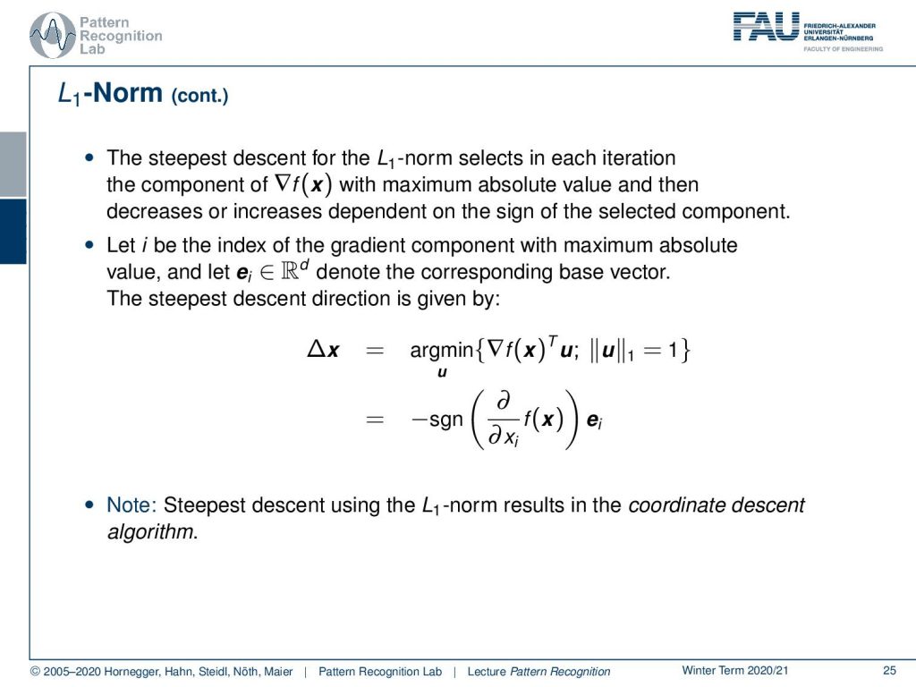
So actually the steepest descent for the L1 norm selects in each iteration the component of our gradient with the maximum absolute value. Then it decreases or increases depending on the sign of each selected component in that direction. So if you define i to be the index of the grading component with maximum absolute value, then we can find some base vectors ei in our d dimensional space that corresponds to this coordinate system. Then the steepest descent direction is simply given as the minimization over u as we’ve seen previously with respect to the L1norm. This then turns out to be simply the sign of the derivative of the function with respect to exactly this coordinate. So this essentially means that the steepest gradient descent using the L1norm results in coordinate descent. So coordinate descent is essentially minimizing according to the L1 norm.
What happens if we take other norms? Let’s look at the maximum norm so here the unit ball looks like this. Now let’s think about the direction of maximum projection and you’ll find it here. So this is the longest projection of our negative gradient direction. Let’s look into another example it will be here. So if we look into maximum norms then we will find update directions that essentially combine several coordinates which will result of course in a different update behavior.
Now we also introduced p norms. So where we have a norm that is essentially described by a matrix. For example, this could be a covariance matrix of a given distribution and if we do this then we generally have unit balls of this ellipsoidal shape. If we want to do this then you will see that the maximum projection will be along this direction here. So this will be our update direction. The major axis of the ellipsoid is crucial for selecting the correct update direction.
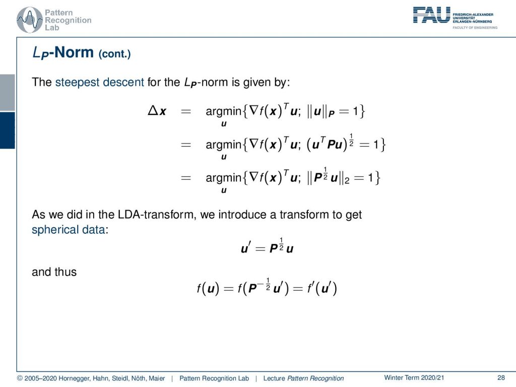
Now let’s look into this in some more detail and then you see that we still use the same idea for finding the minimum. So we take the update direction as the minimum overview as the inner product of our gradient direction with u. But now we are following an Lp norm. Now, this Lp norm we can expand to u transpose Pu to the power of one half. So we need to take the square root of this scalar value and we can rearrange this again then into as we’ve seen also previously in this lecture that we can essentially take a decomposition of P. With this we can then use P to the power of 0.5 times u and the two norm. So if we look at this we can see that these kinds of changes in u we could technically also use as a feature transform. So let’s think about this as a feature transform as an LDA and now we transform into a different space where we take this P 1 over 2 as a transformation matrix to go into some new space u’. So this would be spherical data in which everything is then determined by the L2 norm. If we do so we can see that we can rewrite f(u) as f(P-1/2u’). Then we can find a new definition of f’ that is essentially containing this transform of the features. This gives us f’ and u’. Now we can think about how to minimize the direction in that particular transformed space.
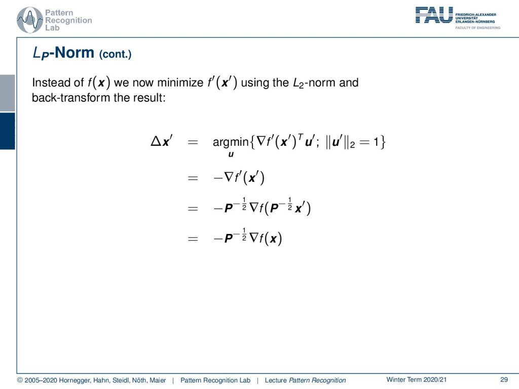
If we do so then we now minimize f’(x’) prime according to the L2 norm. So if we think about this then we can see that this is nothing else than the negative gradient direction of f’(x’). So we know that in the two norms we essentially just have the negative gradient direction. We can reuse this result and now that we’re here we can substitute back so we get our f’ and our x’ replaced. If we do so we see this is a gradient so we also have to apply the chain rule which then gives us our minus one over two times the gradient and the transformed one over two. Now let’s also replace our x’. This will cancel out the inner transform. So here we then have minus P-1/2 times the gradient position at x.
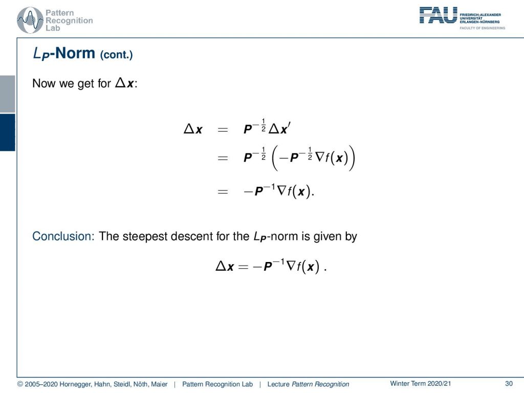
Now let’s see what happens if we apply this to find our update direction ∆x. Here again, we need to apply the P-1/2 and we apply our update direction x’ that is what we already found on the previous slide. So we just plug it in here and then you see that we have essentially two times our P-1/2 and this means we can simplify this entire term to minus P inverse times the gradient direction. So the conclusion is the steepest descent direction in Lp norm is given as the inverse of the P times the gradient direction times -1.
So now we’ve seen different norms let’s look into one more idea in order to perform updates. This is newton’s method so the idea here is that you select a point and then you compute the minimum of the second-order Taylor approximation. Here you see that we have this point then we essentially compute the second-order Taylor approximation and find the minimum. We take this point again take the second-order Taylor approximation and take the minimum again and so on until we actually find the actual minimum.
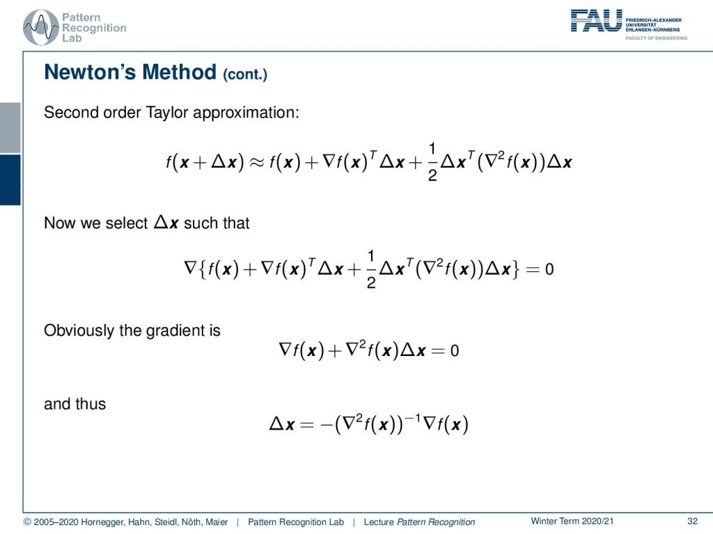
So remember the second-order Taylor approximation is given by f(x) plus the gradient of f(x) transpose delta x plus 1 over 2 and now this quadratic term where we have ∆x transpose times the hessian matrix times ∆x. Now what we want to do is we want to select our update direction such that we essentially get the minimum gradient position. So we need to compute the gradient of our approximation. Let’s do that then you see that the terms that are not associated with ∆x just cancel out. We can now see that we essentially get the gradient at f(x) plus the Hessian matrix times ∆x equals zero. This means we can solve easily and here you see that we get the gradient direction times the inverse of the hessian matrix and multiplied with -1.
So now let’s look at some conclusions newton’s method is an x-dependent steepest descent method regarding the Lp norm where P is simply the hessian matrix. So this is also a pretty nice observation, isn’t it?
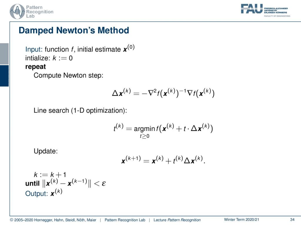
In total, this brings us then to the damn newton’s method. So here we input a function f an initial estimate of x(0) and then we start again with k equals to zero. We compute the newton step. So here we need the hessian matrix inverted at the position x(k) and then we multiply it with the gradient at x(k) and multiply it with -1. So this is the update direction then we do our line search and we can compute the update. We iterate until we have only small changes.
So I hope you learned some lessons here. We’ve seen that we can use different norms for selecting the update direction depending on the norm we get a different update direction. If we take the two norm it’s the negative gradient direction. If we take other norms we have to change the update direction and if we look into Newton’s method we essentially have the update using a p norm where P is given by the Hessian matrix. So this is a very nice observation and with this then we can apply different kinds of decent methods. They are very useful if you want to work on the remaining optimization problems in this class. Of course, you should be aware of the relations of the different optimizers that we discussed here. These are quite crucial observations and I would really have a look at those not just for the exam but I think it’s also relevant for your future career if you want to work in machine learning or pattern recognition then you have to be very familiar with these methods.

So next time in pattern recognition we want to start looking into a really nice method for pattern classification that is the so-called support vector machine.
So I also have some further readings again the book by Boyd and Vandenberghe Convex Optimization is really very good and I can recommend that to everybody. Also, Numerical Optimization is a very good one.
I also prepared some comprehensive questions that may help you in the exam preparation and with this, I can only say I hope you enjoyed this little video and I’m looking forward to seeing you in the next one. Bye-bye!!
If you liked this post, you can find more essays here, more educational material on Machine Learning here, or have a look at our Deep Learning Lecture. I would also appreciate a follow on YouTube, Twitter, Facebook, or LinkedIn in case you want to be informed about more essays, videos, and research in the future. This article is released under the Creative Commons 4.0 Attribution License and can be reprinted and modified if referenced. If you are interested in generating transcripts from video lectures try AutoBlog
References
- S. Boyd, L. Vandenberghe: Convex Optimization, Cambridge University Press, 2004. ☞http://www.stanford.edu/~boyd/cvxbook/
- Jorge Nocedal, Stephen Wright: Numerical Optimization, Springer, New York, 1999.