These are the lecture notes for FAU’s YouTube Lecture “Pattern Recognition“. This is a full transcript of the lecture video & matching slides. We hope, you enjoy this as much as the videos. Of course, this transcript was created with deep learning techniques largely automatically and only minor manual modifications were performed. Try it yourself! If you spot mistakes, please let us know!
Welcome back to Pattern Recognition. Today we want to look into the original formulation of the linear discriminant analysis that is also published under the name Fisher transform.
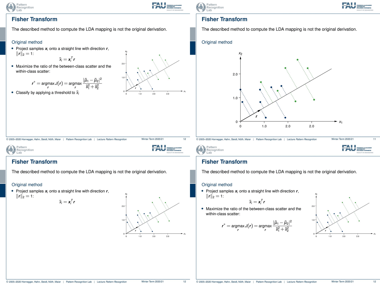
Here we see the original idea that was used to derive the LDA mapping. The original idea is that you want to project onto the direction that is essentially maximizing the class information while minimizing the spread within the classes. This is then introduced as the direction r. Here we stay for the time being with a two-class problem. So we only have classes 1 and 2. Now, how can we do this? Well, we project everything in this ideal direction r. This can, of course, be done by taking the feature vectors and computing the inner product with r. And this then gives us a scalar value x ̃ᵢ. This value has to be determined using r, so r is determined as r*, which is the maximization of the ratio of the between-class scatter and the within-class scatter. You see that the between-class scatter is essentially given as in this two-class case as the subtraction of the means and essentially the two norm of this. And then the within-class scatter is given here by s. s is essentially derived by the covariance of the individual classes, so the scatter within the class. We will see that in a bit. And in the end, we want to apply essentially a threshold on our x ̃. This will tell us to which class to assign the decision.
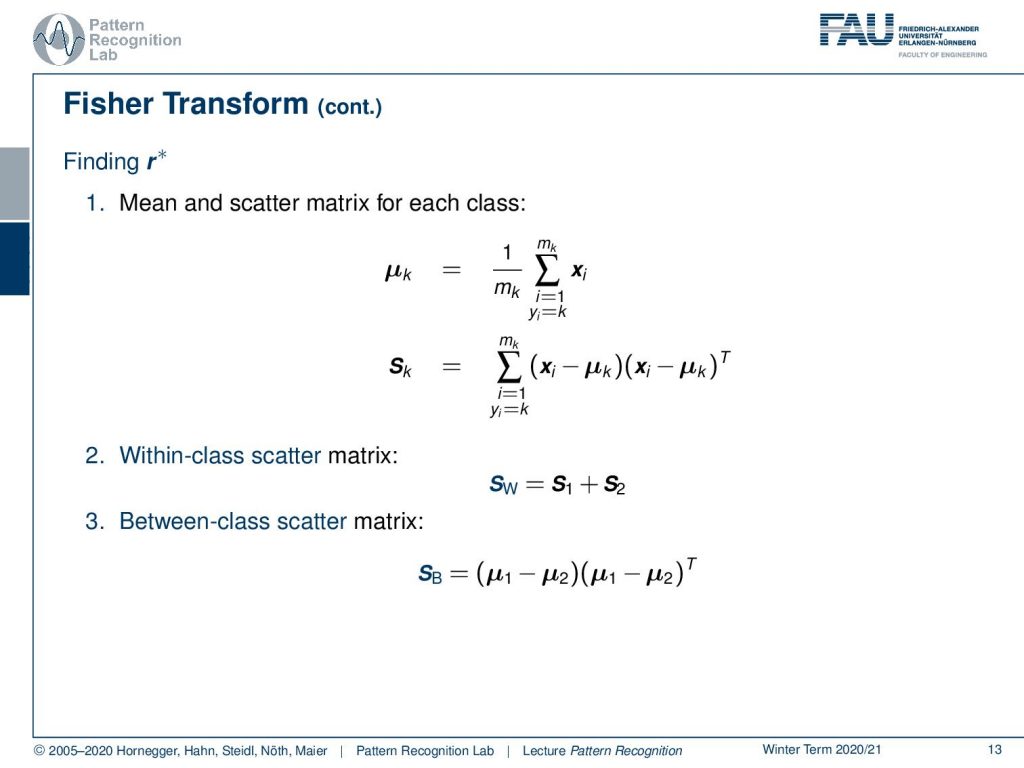
So, what are the steps to compute this? Well, the first thing you do is compute the mean scatter matrix for each class. So you have to know the class membership. Then for the respective class, you can compute the mean value and the scatter matrix that is essentially the covariance matrix within this class. And if you have that, then you can also compute the so-called within-class scatter matrix. This is called sw, and this is essentially the sum of the two within-class scatter matrices. so this is essentially s1 + s2. What we also need is the between-class scatter matrix. and this is given simply as μ1 – μ2. And then the outer product of the same vector that gives you the between-class scatter matrix. Note that this is the simplified version for two classes only. It’s essentially slightly more complex if you want to go towards more classes. Then you essentially end up with the inter and intra-class covariance matrices.
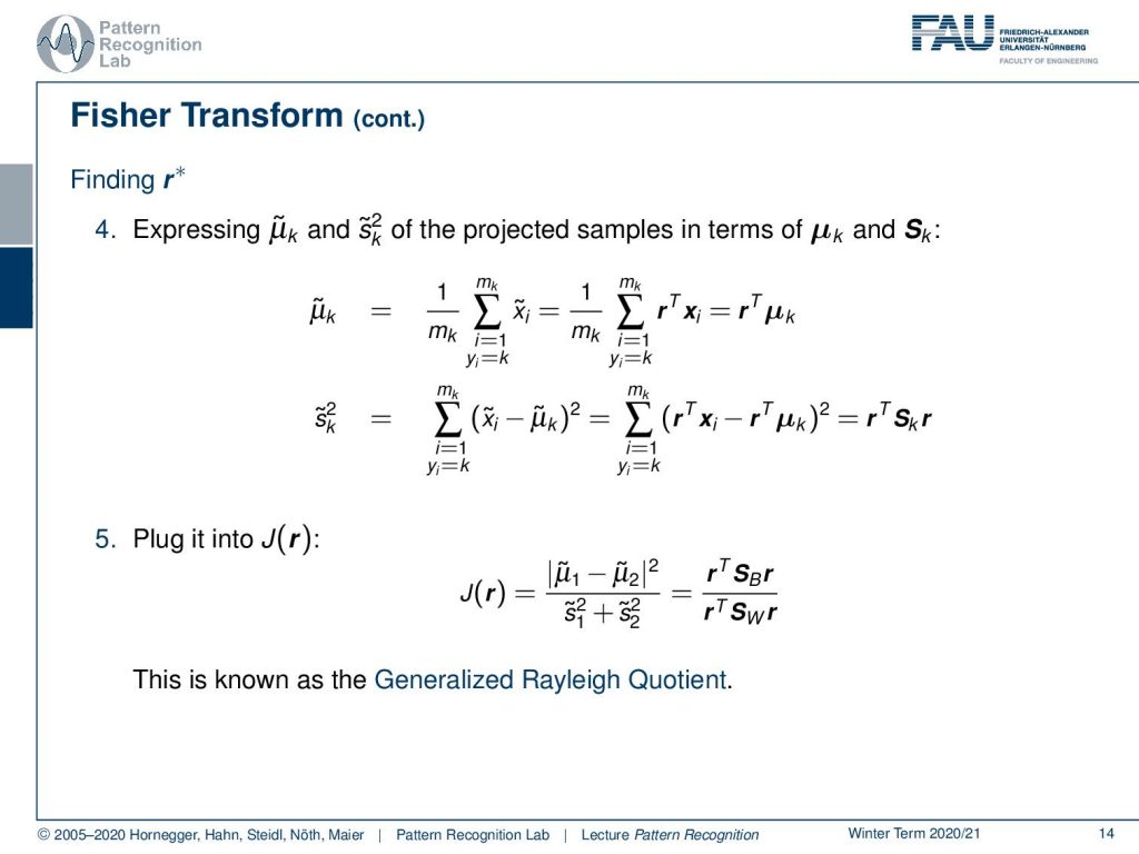
Now, how can we then find r*? r* is essentially used to compute our x tilde. and with x ̃, we can then also find our μ ̃ tilde and s ̃k. Let’s start looking into μ. You see here that this is essentially using r as an inner product. And if we know that this is an inner product, we can see that r is constant over the entire term. So we can compute the mean over the respective class and pull out the rT. Let’s look at the scatter matrix. And here you can see that we actually need to compute the variance in our rT direction. And this can then, essentially, be transformed by applying again our projection onto rT of the individual vectors as well as the means. This then essentially maps back to having nothing else than the respective within scatter matrix multiplied with rT on the left-hand side and r on the right-hand side. Now that we found this, we can plug this into our actual definition of this fraction. This would then simply mean that we have to subtract the two means, and we have to divide by the square of the respective scatter coefficients. Note that this is also known as the Generalized Rayleigh Coefficient. This can be used in order to find rT.
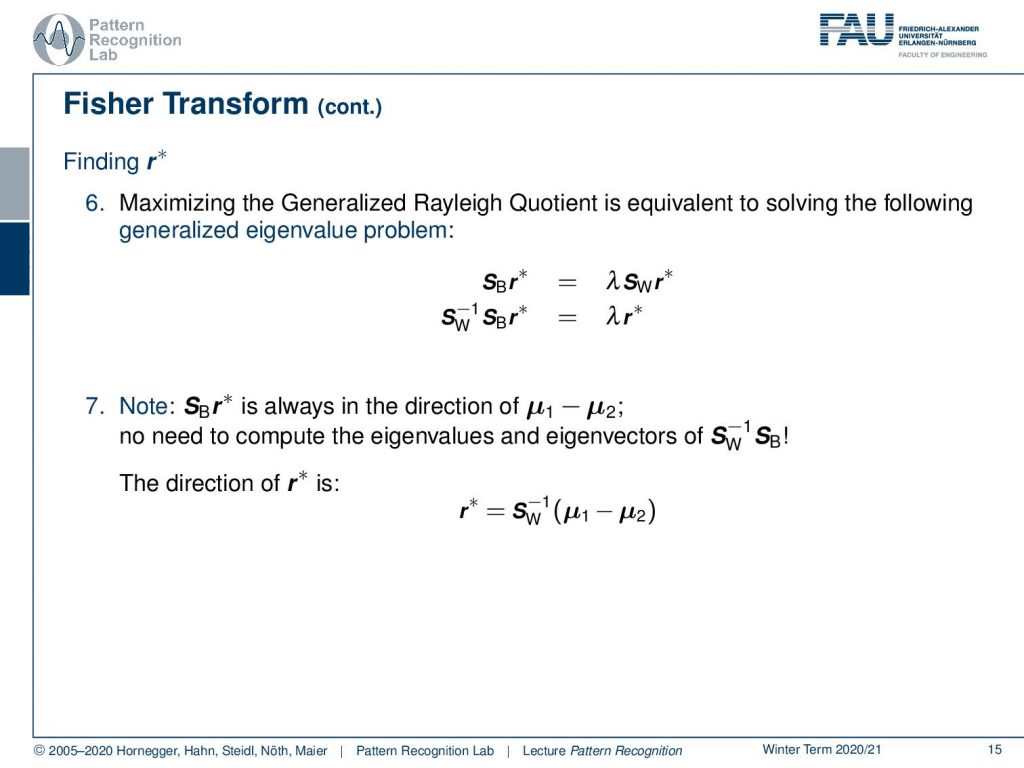
How do we do that? Well, we maximize the Generated Rayleigh Coefficient, and this is equivalent to solving the following generalized eigenvalue problem. We essentially want to have the product of sB r* = λ sw r*. Now we can solve for only one matrix. So we take the inverse of sw and multiply it from the left-hand side. And you see here then that we essentially come up with this matrix that is sw inverse times sB. So this would be the inverse of the within scatter matrix times the between scatter matrix. In this two-class problem, the projection of r* times sB is always in the direction of the two means, as we have already seen in previous videos. This is the decisive direction. So there’s actually no need to compute the eigenvalues and eigenvectors of the matrix in this case. We can simply then compute the direction as the difference between the two means. This, normalized with the inverse of the within scatter matrix, will give us r*.
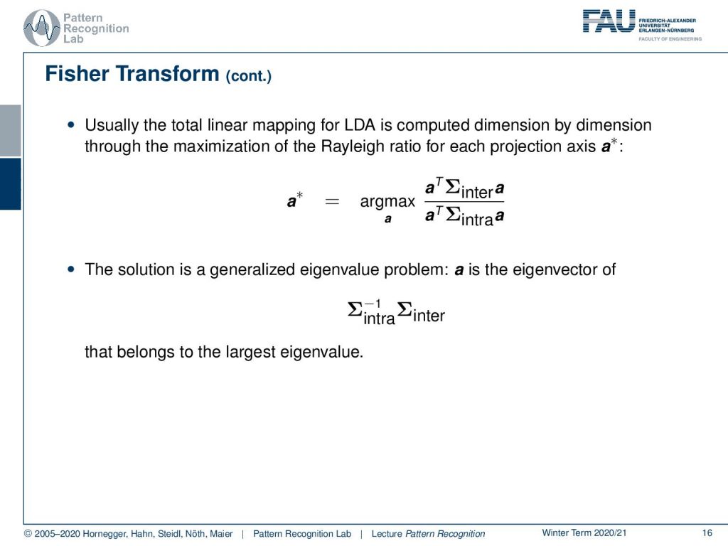
Usually, the total linear mapping for LDA is computed dimension by dimension through maximization of the Rayleigh ratio for each projection direction a*. There we then maximize this for the respective classes, and we always take the inter and intra-scatter matrixes. This can also be found by the solution of a generalized eigenvector problem. a then is the eigenvector of the inverse of the intra-class covariance times the inter-class covariance. And this one then is, of course, found as the largest eigenvalue.
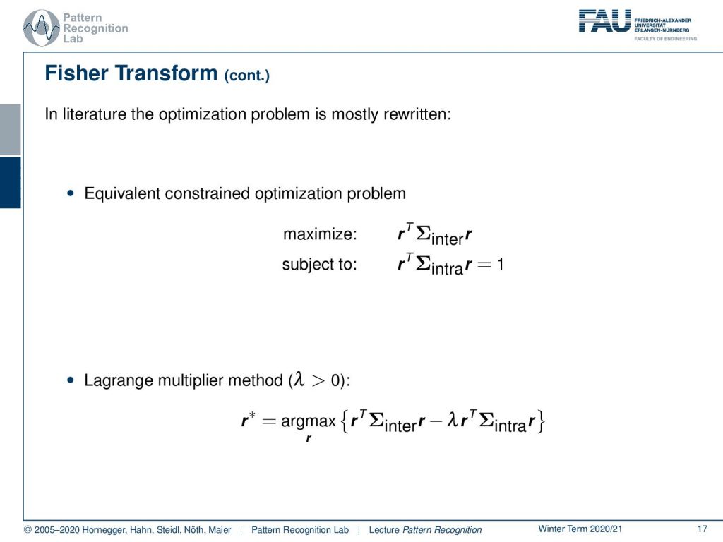
Typically, what you find in literature is the formulation in the following way. So you can also write this up as the equivalent constrained optimization problem. There you maximize rT times the inter-class covariance matrix times r, subject to rT times the intra-class covariance matrix times r equals to 1. So this is essentially again this constraint. And we want to limit the solution space such that we don’t get an optimization problem that would simply have the solution at positive infinity. If you use again the Lagrange multiplier method with λ greater zero, then you can write this up as the maximization of the respective data term that is rT Σinter r minus the Lagrange multiplier rTΣintra r. This is a typical way then how to solve this problem. You can essentially use the solution strategies as you’ve seen on the previous slides also for this kind of Lagrange multiplier method.
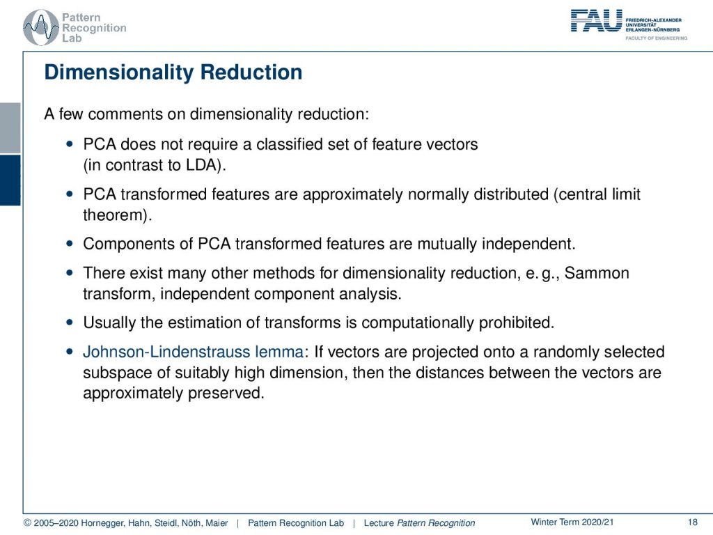
A few comments on dimensionality reduction. PCA does not require a classified set of feature vectors. So PCA can always be applied, you don’t need class memberships. For LDA you have to know the class membership. Otherwise, you won’t be able to compute Φ. The PCA transform features are approximately normally distributed according to the central limit theorem. And the components of PCA transform features are mutually independent. There exist many other methods for dimensionality reduction. For example, the summon transform and the independent component analysis. So this is one choice of feature methods. Usually, the estimation of these transforms is computationally quite expensive. The Johnson-Lindenstrauss lemma tells us if vectors are projected onto a randomly selected subspace of suitably high dimension, then the distances between the vectors are approximately preserved. This is also something that is quite commonly being used, the projection onto random subspaces.

This already concludes our introduction to the linear discriminant analysis. You’ve seen now the rank reduced version, and you’ve seen the original transform introduced as Fisher transform. In the next video, we want to talk a bit about the applications where this can actually be employed and how these methods can be used in various application scenarios of Pattern Recognition. Thank you very much for listening, I’m looking forward to seeing you in the next video. Bye-bye!
If you liked this post, you can find more essays here, more educational material on Machine Learning here, or have a look at our Deep Learning Lecture. I would also appreciate a follow on YouTube, Twitter, Facebook, or LinkedIn in case you want to be informed about more essays, videos, and research in the future. This article is released under the Creative Commons 4.0 Attribution License and can be reprinted and modified if referenced. If you are interested in generating transcripts from video lectures try AutoBlog.
References
Lloyd N. Trefethen, David Bau III: Numerical Linear Algebra, SIAM, Philadelphia, 1997.
T. Hastie, R. Tibshirani, and J. Friedman: The Elements of Statistical Learning – Data Mining, Inference, and Prediction. 2nd edition, Springer, New York, 2009.
B. Eskofier, F. Hönig, P. Kühner: Classification of Perceived Running Fatigue in Digital Sports, Proceedings of the 19th International Conference on Pattern Recognition (ICPR 2008), Tampa, Florida, U. S. A., 2008M. Spiegel, D. Hahn, V. Daum, J. Wasza, J. Hornegger: Segmentation of kidneys using a new active shape model generation technique based on non-rigid image registration, Computerized Medical Imaging

