Lecture Notes in Pattern Recognition: The Big Picture

These are the lecture notes for FAU’s YouTube Lecture “Pattern Recognition“. This is a full transcript of the lecture video & matching slides. We hope, you enjoy this as much as the videos. Of course, this transcript was created with deep learning techniques largely automatically and only minor manual modifications were performed. Try it yourself! If you spot mistakes, please let us know!
Welcome, everybody! Today I want to answer a couple of questions that you have been asking over the last couple of weeks. They’re of course all regarding our lecture Pattern Recognition. Some of you had a bit of trouble following the short videos because we have around one proof or one chain of argument in a video, but sometimes it’s difficult to preserve the entire overview over the complete lecture. For these reasons I prepared a short video here where we’re summarizing the entire content of the lecture and give a quick summary of everything that will happen in this course.
Okay, so Pattern Recognition “the big picture”. Of course, you want to learn python and machine learning and pattern recognition all of those things. I guess this is also one of the reasons why you’re watching this video. But then again, some of you might not be so eager to learn the math. I think this is still a set of skills that you may want to be able to acquire because many of you do this course here because they want to work as a data scientist or a researcher in artificial intelligence later on. So I think math is still something that you should be aware of. And believe me, this math is not too hard.
Of course, machine learning is kind of difficult to access if you don’t know the math, this is why we also provide now extra videos where we explain the basics of math that are fundamental to follow our course.
But let’s say it’s not just that you have to be good at math, but it’s actually all about function fitting and matrix multiplication. These are essentially the key techniques that you need for this course, and also for a career in machine learning. So you don’t have to follow all of the topics of math, there’s a couple of things that you have to know by heart, and these are also the ones that we will emphasize in the additional videos that we now provide.
Now, what’s the big picture? Our class is of course “Pattern Recognition”, so here is our pattern recognition cloud, and these are the topics that we are discussing. We start with an introduction, we start with classification, and introduce why we need this. So this is essential to be able to derive a decision from some input data. We do that with the pattern recognition pipeline. The pipeline starts with the sensor, which is digitized then we extract features. Finally, after we have found suitable features, we go ahead and then train a classifier. Now, this class is mainly about the classifiers and not so much about feature extraction. We have another course “Introduction to Pattern Recognition” where we talk more about the sensors and suitable features for certain tasks. Then we also introduce evaluation measures, but we only talk about them very little. So don’t be afraid, this is not too relevant if you want to prepare, for example, for our examination. But of course, you need to know about classifiers and how to evaluate them because this will be key for your career. So we have only a very course overview over different evaluation measures here.
Then, we go ahead to the basics. We review the base theorem and have a small example about that, so I think this should be very useful. And then we go ahead and talk about the Bayes classifier. The Bayes classifier is a concept that stems from the Bayes rule. The Bayesian classifier is the optimal classifier if we follow a zero-one loss function and we have forced decision. So these are two key concepts for our class. Remember, for the base classifier we didn’t specify how to get the distribution of the classes. This is also something we talk about in detail in the remaining class. This is an idealized concept where all of your assumptions have to match the underlying data. then We also had a short view at linear algebra. I can tell you if you want to follow this course, I definitely recommend watching another lecture of me where we introduce matrix calculus, singular value decomposition, and other fundamental concepts of linear algebra that are important for this class. If you don’t like the rather old recording that much I might be inclined to do a new version in this new style of this video. Maybe if you send me a message or if you show that there’s interest in this I would probably do it. Then we also had a couple of basics in optimization, in particular, constraint optimization is a very important concept for this class. I already decided that I will make another video about Lagrangian approaches and how to set up Lagrangian functions and how this optimization works. So you will see that very shortly.
Then we started discussing logistic regression. Now logistic regression is a concept where we essentially show that we can convert a generative modeling approach into a discriminative and a discriminative into a generative one. So a generative approach will model the classes class by class and their probability distributions, and the discriminative will directly involve modeling of the decision boundary. We’ve seen that if we start with generative models, then we can convert them into a decision boundary by computing the position, where the probabilities of for example two classes are equal. Then at this point, the decision boundary is found, and here you switch from one class to another. If you use the logistic function, the sigmoid function, then you can also start with a decision boundary and you can create from that the distribution of the individual classes. So if you use the sigmoid function, then you can actually create again a distribution for a specific class that is only determined by the decision boundary. That is a pretty useful concept. Then we have seen that essentially, the classification problem can be expressed as a regression problem. Then we also looked into the exponential family. Now the exponential family is a very nice collection of probability mass and density functions. We have seen that they have the property if the dispersion parameter is equal, then the decision boundary is modeled as a line. This is very useful for the case of Gaussian distributions. We have seen if the covariance is identical, then also the decision boundary will be a line. Also, a very useful tool is the log-likelihood function. We’ve seen that if we apply the logarithmic function, then the position of the maximum doesn’t change. So we can use that to simplify our estimation problems. We’ve seen that with many of the probability mass and density functions if we apply the logarithm, then actually the exponential function goes away and we end up back to problems that we can tackle with linear algebra. This actually happens quite frequently in this class.
We went further on for the naive Bayes. The naive Bayes is a rather simple method, and it essentially assumes that all of the dimensions are independent. With this assumption you can build efficient classifiers very quickly.
Furthermore, we discussed linear discriminant analysis. Now, linear discriminant analysis is essentially a feature transform. But here you assume to know the membership to the classes and then you try to find a linear transform that optimally separates the classes while minimizing the scatter within the class. We’ve seen the whole story until we find this. So for example, if we were able to find a space in which all of our classes have a uniform covariance matrix, then all of our decision boundaries would be lines. And in this space, we could use k-1 dimensions to be able to separate all the classes from each other. Furthermore, we would then be able in the space to also model very high dimensional feature vectors in a much lower dimensional space. And we would not lose any information by this dimensionality reduction given that the classes have a Gaussian distribution and so on. So there’s a couple of side constraints to this, but generally, this is a very useful transform and we’ve seen two different variants of this: the whitening transform and the sphere data and its properties. So this is when all of the classes have a uniform covariance matrix. We’ve also seen the rank reduced LDA and the original Fisher transform. Furthermore, we looked into some applications. The applications were mainly the adidas_1, which is a shoe that has an embedded classification system. So LDA-type of approaches and those simple classifiers are so computationally inexpensive that they can run on the embedded hardware even of the shoe. This was a pretty cool thing and that has been developed by my colleagues Joachim Hornegger and Björn Eskofier, and it was actually developed into a product. We also looked into principal components and how we can do segmentation of complex structures that have a high degree of variability. There we’ve seen active shape models that are pretty frequently used in medical imaging for image segmentation.
Furthermore, we then went ahead with regularization and norms. Now regularization is a very important concept that we also use many many many times in this class. And with regularization, we can essentially avoid numerically unstable solutions, and we can also force our solutions to have desired properties. We have in particular seen the example of Tikhonov regularization for regression. There we then can essentially demonstrate that the Tikhonov regularization is identical to statistical assumptions where we assume that we have an additional prior. This prior then relates directly to the additional norm on the properties of our regression. This was extremely useful. Then we looked into different norms, the L1-norm, the L2-norm, and their properties. This can then even be expanded to find sparse solutions. And then, these schemes of finding sparse solutions give rise to the entire domain of compressive sensing which we’re not discussing in detail in this class. If you’re interested in that you could attend one of our medical imaging classes where we go into much more detail about these things. So, regularized regression where we have specific properties then embedded into the solution. We discussed the norms as I already said, and then norm dependent regression. There, you’ve seen that the norm dependent regression then has specific properties such as sparseness. Furthermore, we looked into different penalty functions, and these penalty functions are essentially a variant of norms. Here you can then see that we can design them in a way that they also have specific properties. In particular, there is are also functions like the Huber function which is an approximation of L1-norm that is completely differentiable. So we don’t have any discontinuities in the gradient, which is very useful if you’re following a gradient descent procedure.
Furthermore, we then looked into perceptrons and multi-layer perceptrons. So, the simple perceptron by Rosenblatt and the convergence proofs and how many iterations you have actually seen. And the very important point about this lecture is that we see that the space in between the classes is a key factor for the number of iterations that you actually need in order to find the point of convergence for the Rosenblatt perceptron. And you’ll see that this separation of the classes, the margin, will come again also in other classifiers. Then, we did a short excursion to multi-layer perceptrons because, of course, deep learning is now a very important field of research and you should at least have seen the classical approach of the multi-layer perceptron. But if you’re interested in these topics I really recommend to attend our lecture “Deep Learning”.
Then, we went ahead towards further optimization. And here in particular we started looking into convex optimization and some of these properties. Convex optimization is a key concept also in this class which we will see in the next couple of classifiers. Then we have seen a method to efficiently solve optimization problems that is the line search. And we have seen that the search direction, so following the steepest descent direction, is not necessarily always the gradient direction. If you use a specific norm this may alter the gradient direction and here we talk then about normal dependent gradients. And we’ve seen that if you have an L2– norm everything is fine, so it’s just the gradient direction. But if you work with L1 or other norms, then suddenly the direction of steepest descent changes.
This then gives rise to looking into support vector machines. Now in support vector machines, we had the hard margin case where we essentially maximize the margin, this gap between the two classes, and we try to find the decision boundary that is optimal for the spacing between the two classes. This will only find convergence in the case that the classes are separable. This is why they then introduce the soft margin case where we have slack variables that allow us to move misclassifications again to the right side of the decision boundary. And then we also have a problem that we can also solve even if it’s non-separable. We also looked into the Lagrange dual function, and this then gave rise to the notion of support vectors. So we have seen that in the Lagrange duo we can express the entire optimization only for Lagrange variables. So, all the primary variables like the normal of the decision boundary and so on cancel out in the dual function. And if strong duality is given, the solution to the dual will also give us the solution to the primal which is kind of a very interesting property. We can then use this in the support vector machines. And we have seen that essentially we only need those vectors that lie on the margin of the decision boundary to determine it. And all of the other vectors from the training data we don’t need anymore. These vectors are the support vectors. And these are all vectors that have a non-zero Lagrange multiplier. Furthermore, we’ve seen that kernels are an important concept. So with kernels, we can map inner products into a higher dimensional space. We don’t even have to define the actual mapping into the space, as long as we’re able to evaluate the inner product. We’ve also seen that if you use the kernel trick, then even determining the decision boundary of a new observation doesn’t even require the actual transform to this kernel space. But you can express everything within the inner products of this kernel of space. That’s also a very useful property.
We further then go ahead to EM algorithm, the Expectation Maximization algorithm, which is a key concept if you have hidden variables. We then show this in the so-called Gaussian mixture models where we then also have to estimate the parameters of several Gaussian functions and their mixture. This can be very well expressed using the EM algorithm. And we’ve seen also that this concept can be extended to many many more applications.
Furthermore we looked into the independent component analysis. Now, independent component analysis is a feature transform again. But this feature transform doesn’t require the class membership. Instead, we require to know something about the distribution of the features. So we assume that the features that we observe are independent. We have multiple features that we observe and they can be mapped into a space that fulfills the property of them being independent. And we have also seen that if we have these approaches that we can do cool things like separating different sources blindly. So superposition of images or sounds can be separated with the independent component analysis. We’ve also seen that the most random distribution with a fixed standard deviation is actually the gaussian distribution. And if we assume non-Gaussianity, then we can figure out the original components if they are not Gaussian distributed. So if everything were distributed Gaussian, then we are not able to identify the independent components. Very well!
Then we looked essentially into which of the classifiers is now the best one, and we found that there is the no free lunch theorem. So if you don’t know anything about the problem, then you cannot determine the best classifier per se because the performance of different classifiers may be very different on different problems. Also, we’ve seen the bias-variance trade-off that tells us that if you increase the number of parameters, the complexity of your classification system, you may fit the training data very well, but this close fit on the training data may lead to poor performance on the test data set. And this is because any bias, any error in the training data set can be compensated by just including enough variance in the classifier. But the main problem with this is that it may then very easily lead to overfitting. And we shortly discuss topics of how to estimate parameters on finite data sets. But I think the main concept that you should take from this is the concept of cross-validation, jackknifing, and so on. We just discussed them because you should have heard about those concepts.
The Last topic of the lecture is boosting. Now boosting has the idea of combining many classifiers and it has been a very popular technique. In particular, it has been used a lot in the so-called Adaboost algorithm. So in the Adaboost algorithm, you essentially train a classifier after each other. You do a first round of classifiers, train it, and then you start a re-weighting of the instances that have been misclassified. Then you train a new classifier and you iterate until you have a fixed number of classifiers. And then in the end you choose the optimal configuration of their weightings to determine the final classification result. And you could argue that you then have kind of let’s say 50 different classifiers and they do more or less independent assessments. The final prediction is then given as the optimal combination of those 50 classifiers, so we try to use essentially the wisdom of the crowd. This can be done with boosting. And in particular, Adaboost is an important method. It has then led to the development of the so-called Viola Jones algorithm which is a very popular face detector that you can find today on many smartphones, on cameras, and so on. When they automatically detect the faces it’s using the Viola Jones algorithm that we show in this part of the lecture. Okay, so this is already the big picture! you see that we are essentially running through different kinds of classifiers. We start with the simpler ones, but we always have the optimization and the math in the back to understand the more complicated methods. And then at some point, we run out of time, so we stop with boosting. There would be more interesting methods that we could look at. And of course, these methods are the traditional classical methods and today many methods now employ deep learning. But what you’ll find if you discuss deep learning, if we look into the details, essentially all of the concepts that we deal with in this class, they come again, just in different flavors. But we use constrained optimization, we use concepts of convexity, we use non-convexity or local convexity, and of course, we also use a lot of linear algebra. So these concepts are very important. You see here now how things developed over the years in machine learning and pattern recognition, but these concepts are not outdated. You still need them for many of the modern-day techniques.
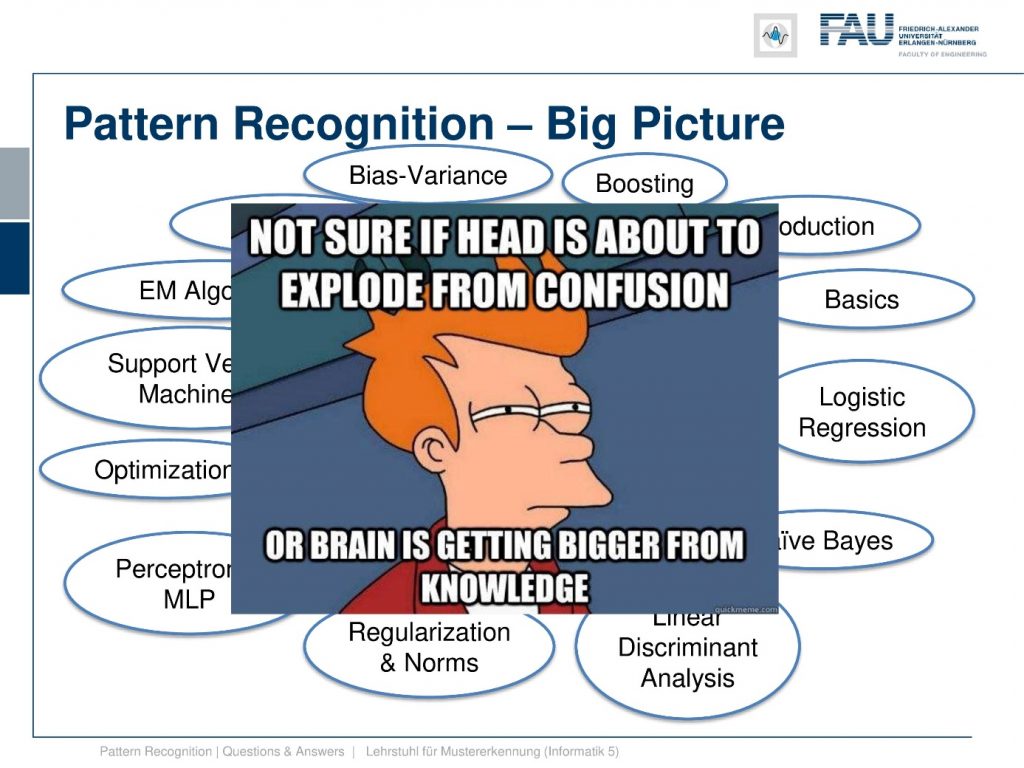
I know this is a lot of math, so please have a look at the things. If you have trouble with understanding what I’m talking about send your questions, I will answer them. We have different comment functionalities where you can interact with us. There are many, many ways to engage with us, so please use them and don’t let your head explode. But let’s hope that you really get the knowledge into your heads such that you can then go ahead and become a machine learning expert and maybe at some point a data scientist.
And keep in mind: when people advertise, they typically claim it’s artificial intelligence, when they hire they want to experts in machine learning. But when you finally then implement the stuff, it’s probably linear regression.
Thank you for your attention! I hope you enjoyed this little video and it helps you with understanding what the main ideas of this class are. And of course, as I already said, please ask your questions. If there are questions that appear again and it takes a little longer to answer them I’m also very happy to produce more videos of this kind. And you will see we already gathered quite a few of those questions and try to answer them in an appropriate way such that you can follow the contents of the lecture more easily. Also, in cases, if you are not so super aware of the mathematical concepts. I’m trying to pull up some refresher courses here such that you get more easily into the math. I hope you enjoyed this little video and I’m very much looking forward to meeting you again in one of my other videos! Thank you very much for watching and bye-bye.
If you liked this post, you can find more essays here, more educational material on Machine Learning here, or have a look at our Deep Learning Lecture. I would also appreciate a follow on YouTube, Twitter, Facebook, or LinkedIn in case you want to be informed about more essays, videos, and research in the future. This article is released under the Creative Commons 4.0 Attribution License and can be reprinted and modified if referenced. If you are interested in generating transcripts from video lectures try AutoBlog.