Lecture Notes in Pattern Recognition: Episode 5 – The Logistic Function

These are the lecture notes for FAU’s YouTube Lecture “Pattern Recognition“. This is a full transcript of the lecture video & matching slides. We hope, you enjoy this as much as the videos. Of course, this transcript was created with deep learning techniques largely automatically and only minor manual modifications were performed. Try it yourself! If you spot mistakes, please let us know!
Welcome back to pattern recognition. Today we want to start looking into more details on how to model the classifiers and the different decision boundaries. We’ll start with the example of logistic regression.
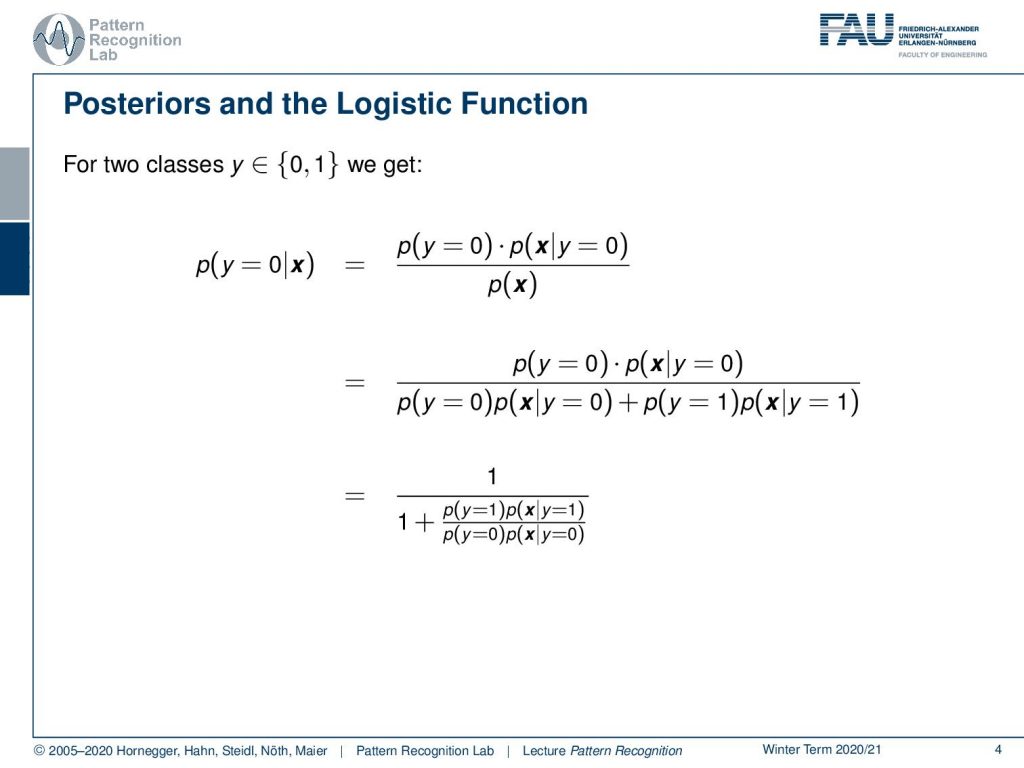
Logistic regression is a discriminative model because it models the posterior probabilities directly. So, we can essentially have a look at our posterior probability. Let’s say we have two classes that are encoded as zero and one and now we want to compute the probability of observing zero given some observation x. Now we know that we can apply Bayes theorem and therefore we can rewrite the probability in the following way. So, we have the probability of observing zero at all and then we have the probability of the observation given a particular class and we divide by the probability of observing x at all. Now we can essentially use this trick here where we do the marginalization of x. So, we know that this is also expressible as the sum over the joint probabilities. Here we already replaced the joint probabilities with the respective composition with the priors and the constraint probability. You can see that we essentially then replace it with the sum in the denominator. Now we can rearrange this a little bit by dividing the whole fraction with p(y=0) times p(x|y=0) and if we do so we can get the following rearrangement and you see that we end up with these double fraction. We see that we essentially have the class conditional probabilities and the priors, now all in the denominator.
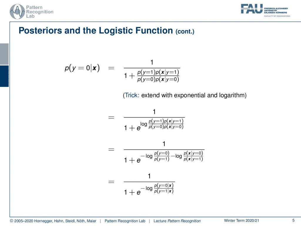
We can further rearrange this a little bit and the idea now is that we want to extend with the exponential and the logarithm. So, if we do so we get the following kind of relation we essentially have the same term and we take e to the power of a logarithm. This would essentially cancel out again to be one. So, this doesn’t change anything and now we can do another trick. We can use the logarithm to split the two and then you would see that we can now rearrange into a fraction of the prior probabilities. We can rearrange into a fraction of the class conditional probabilities. Also, we can observe that we are essentially using the Bayes rule here so we can also rearrange it to the following equation rather than simply have the fraction of the posterior probabilities. So, this would be equivalent in our case.
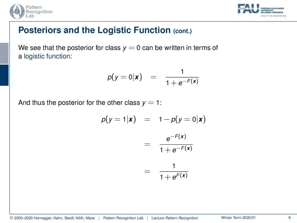
You see that we found a way to rearrange our probability of y equals to zero given x and we found a very interesting formulation here. We can see that this particular shape is actually called the logistic function. So, the logistic function is given as 1 over 1 plus e-F(x) and here F(x) is actually the decision boundary. So, we can see that if we do the same for the other class where y equals to 1, we get the following relationship. We have 1 minus p(y=0|x) and now we can essentially plug in our previous definition and rearrange a little bit. You can see now that we essentially can simplify this in another step and we get again a logistic function but now with eF(x) in the denominator. So, you see we essentially have two times the same formulation the same function F(x) and on the one side it’s minus F(x) and on the other side, it is F(x). So, this essentially means that F(x) is describing how the probability is being assigned and this is essentially nothing else than the decision boundary. We will look into a little more detail in the next couple of slides.
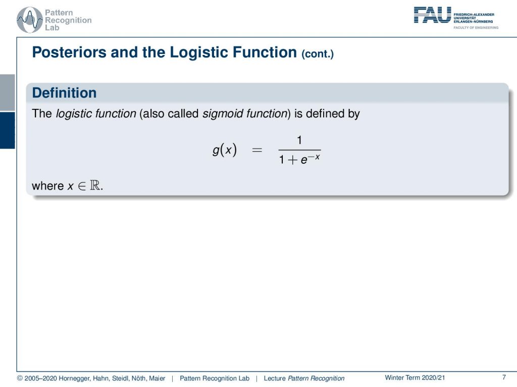
So, we can see that the logistic function which is also called the sigmoid function can be defined in the following way: so it’s 1 over 1 plus e-x and x is simply a real number.
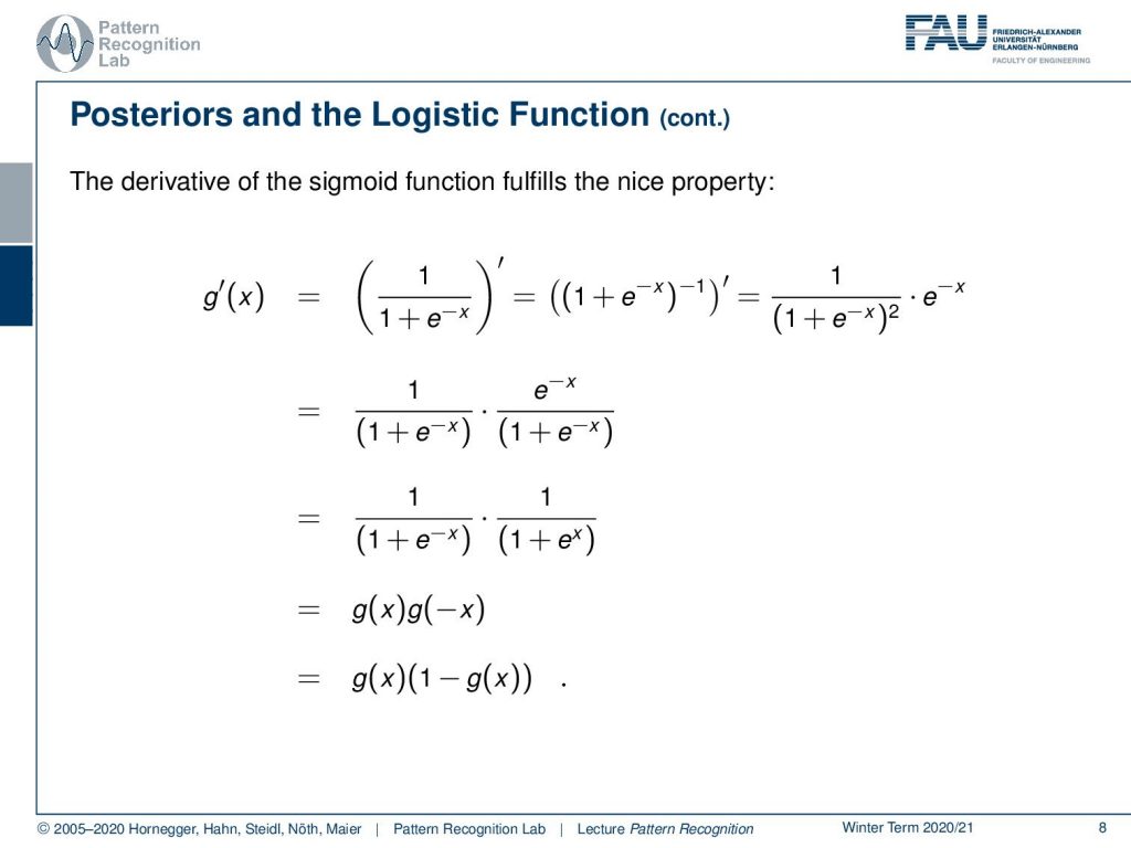
So, this is a very nice function and you see that the derivative of the logistic function fulfills the following property. We can indicate this with the prime here. So, g‘(x) is given as the derivative of the definition of g‘(x). Now we rearrange this a little bit so we express the fraction by essentially writing the entire denominator with to the power of -1 and now we can apply essentially the rules of differentiation. So, we have to reduce the exponent by 1 which then essentially yields 1 over 1 plus e-x to the power of 2 times e-x. So, this is simply the application of the chain rule here. Then we can rearrange this a little bit and write this in the following way and we essentially split the square in the denominator. Then we see that we can then rearrange by flipping the x in the exponent and the right hand term. The next thing that we observe is that the first term is nothing else than g(x) and the second term is nothing else than g(-x). Now we can still rearrange it a little bit because we know that our function is only defined between 0 and 1. So, this is a property of the sigmoid function and this means that we can essentially describe the derivative of our logistic function as the logistic function times 1 minus the logistic function. so this is a very nice property and we will use it actually quite heavily whenever we use gradients of our logistic functions.
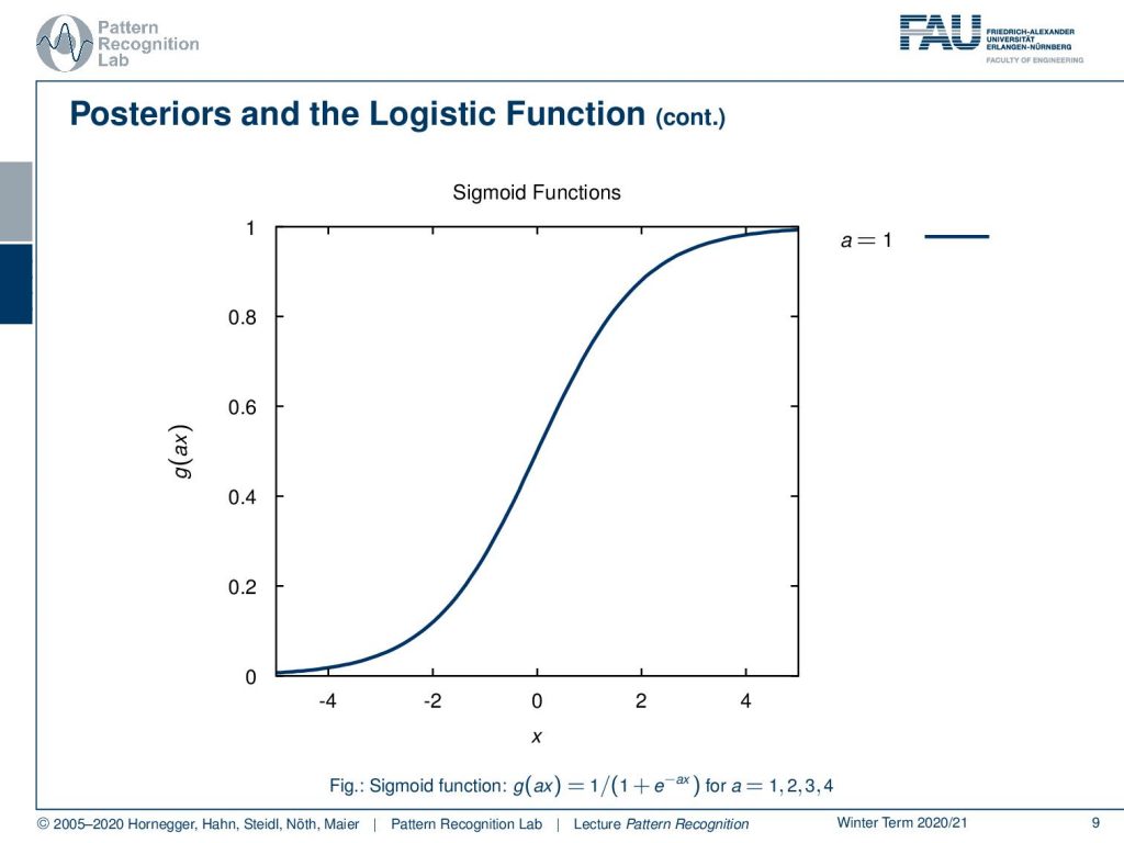
Now let’s have a look at how these functions look like. We can parametrize this with an additional a and this a is then essentially amplifying the magnitude of x and if we now increase a, you see that our sigmoid functions get steeper and steeper.
So, this is actually a quite interesting observation that we’re able to rearrange the probability of a class given a certain observation in this kind of logistic function. We will reuse this observation in the next video. We will then actually look at an example we want to use a gaussian and compute the logistic function together with the gaussian.

So, I hope you enjoyed this little video with a small introduction to the logistic function and looking forward to examining an example in the next video. Thank you very much for listening and see you in the next video. bye bye!!
If you liked this post, you can find more essays here, more educational material on Machine Learning here, or have a look at our Deep Learning Lecture. I would also appreciate a follow on YouTube, Twitter, Facebook, or LinkedIn in case you want to be informed about more essays, videos, and research in the future. This article is released under the Creative Commons 4.0 Attribution License and can be reprinted and modified if referenced. If you are interested in generating transcripts from video lectures try AutoBlog.
References
- Trevor Hastie, Robert Tibshirani, Jerome Friedman: The Elements of Statistical Learning – Data Mining, Inference, and Prediction, 2nd edition, Springer, New York, 2009
- David W. Hosmer, Stanley Lemeshow: Applied Logistic Regression, 2nd Edition, John Wiley & Sons, Hoboken, 2000.